Statistics_2_Revision_short_notes
Year: Specimen • Views: 1 • Downloads: 2



📄 Exam Questions & Readable Text Transcript
Full OCR-extracted text of questions, syllabus codes, and exam instructions.
Extracted Content: Statistics_2_Revision_short_notes
Page 1
Extracted Text
Statistics 2Revision Notes
J une 2016
---
Page 2
Extracted Text
$2 JUNE 2016 SDB---
Page 3
Extracted Text
Statistics 21 The Binomial distribution 5
Factorial... ceeesesesesesssescsecesesecesesecesesscesesecesesecesesesesesecscececesscucscscscecceeeseceseeeeeseeeenseeeeneeeeenees 5
COMPINALIONS .0..... eee esesesesesecececececesecesececesesecesesecesesececeeccececeseseceseseceseseceseseeeseseeeseeeenseeteneeetenees 5
Properties Of "Cy .ceccecsecsecsessessessessessesseesessessssssesssessesecsecsecsucsessecsessessussessscsucsecsecseesesessesseeseeseeseeseesesseeseeseeaeensens 5
Binomial THeOrem uu... eeesecssesscssesecesececesesecesesesesesesecesecescsesesececeeeeeceesecneeseceseeeeeseeeeneeeeeneeeeenees 6
Binomial CoeffiCients .........cecessececsecsesesecsescsessesesscsecsecsesecsesecsesesueseeseseceesesueseceesecaeseseesecueaeeesaeceeaeceeseeeeaeeeeaeeeeaeees 6
Binomial coefficients and CombINALIONS ..........cseesessecessecesseseeseseseesesececseceesecueseceeseceeseeeeaeeeeseceeseceeaeeeeseeeeaeeeeaeee 6
Binomial distribution B(0, )..... ce esssesesssesssssesesecesscsseseceseseceseseeeseseeeeeseeeseseeeseeeeeeeeseneeeeenees 6
Conditions for a Binomial Distribution... ceecsssesseseeseseesesecseseesesecsesecseseesesecsesecaesecaeseesesecaeseeaeaeeeeaeeaeaeeneaeees 6
Binomial Gistribution......... es eesessesesseseeseseeseseesecseseesesecsesecsesecsesecsesecseseceesecueseceeseceeseceesecuesecseaecaeseceeseeeeaeeaeaeeaeaeees 7
Cumulative binomial probability tables
Mean and variance of the binomial Gistribution. 20.0.0... ..eseeecseseeseseesesecseseesesecseseeseseeaeseeeeseesesecaeseeseseeaeseeaeaeeaeaeees 9
2 The Poisson distribution 10
Conditions for a Poisson Gistriutin........eeeeseseseseseseseceseseceseseceseseceseseceseseceseseseseseeeseseeeeeeeees 10
POISSON CISHADUMION..... eee eesesesesesececececesececeseseceseseceseseceseseceseseceseseceseseceseseseseseseseseeeseseetseeeees
Mean and variance of the Poisson distribution. .
The Poisson as an approximation to the binomial ..........cccsssssssssesesseseseseseseseseseseseseseseseseeesens 13
Binomial B(n, p) formal poo. eeesessssesseecesseceesecesecsesecseseceesesseseceeseesesecsesecaeseceeseeeeseeaeseeseaeeeaeeeaeeeeaeees 13
Selecting the appropriate distribution... esssssseseteesesesesesesesesesesesesesesesesesesesesesesesesenenens 14
3. Continuous random variables 15
---
Page 4
Extracted Text
5 Normal Approximations 23The normal approximation to the binomial Gistriution.......... cc cseseeseeeeesecesesesesesesesesesesenee 23
Conditions for apprOxiMAtion. 0.0... eececessecessececseccsececseescsececsecscseesesscsesscsessesesseseeuesecueaesseaeeueaeeaeaeceaeeseaeeeaeeeeaees 23
Continuity COMeCHON .......essecsesecsesessesessesessesecsessesesscsessesesucaessesessesesseaessesessesesseseesesesueaeceesecueaeseeaeceeaeeueaeeeaeeneaees 23
The normal approximation to the Poisson GistrH bution... ccesssseeeeseesesecesesesesesesesesesesenes 24
Conditions for approximation 0... eeseseesesseseeseseeseseeseseesesscsesecsesscsecsesesucaesseaessesesuesecueaesuesecueaeseeseceeaeeeaeeeaeeeeaees 24
Continuity COMeCHON .......essecsesecsesessesessesessesecsessesesscsessesesucaessesessesesseaessesessesesseseesesesueaeceesecueaeseeaeceeaeeueaeeeaeeneaees 24
6 Populations and sampling 25
Words and their mearingS...........essecsssecessecssseceesecsesecsesecsesecsesecsesecsesecsesecsesecseseesesecseseesesecaeseeaeseeaeseeaeeeeaeaeeaeaeae 25
Advantages and disadvantages of taking & CONSUS......sessscssecsseseseceseceseesssecsesecsesecseseeseseeaeseeaeseeaeseeaeaeeaeaeaee 26
Advantages and disaclvantages Of Sarypling...........:ecsssscsssecsssecesseceesecsesecsesecsesecsesecseseeseseeaeseeaeseeseseeaeaeeaeaeeaeaeaee 26
Sampling Gist butions... cssssssssessssseseseescsesescseseseseseseseseseseseseseseseseseseseseseceseseneseseseseseseaenes 27
7 Hypothesis tests 28
Null and altemative hypotheses, Hp and Hy... eeesssesssssesecsseseceseseceseseceseseseseseeeeeseeeeeeeeeeeeeeeee 28
Hypotheses and significance level
Critical regions and significance levels... eeesssesessseseceseseceseseceseseceseseseseseceseseeeseseeeseeeeeeeeeeeee 29
Poisson and Binomial .0.......ccssessssessssecsesesseseeseseesesecsesecsesseaesucsessesessesessesesaeaessesessesecaeaeseeaeeeeaeseeaeceeaeeeaeeeaeeneaees 29
One-tail and two-tail t6StS...... ce eeeecsseseseseseceseseceseseceseseceseseceseseseseseceseseceseseceseseeeseseeeeeseeeeeeeeeee 30
Worked examples (binomial, one-tail test) 0.0... ccescecessecessecesseceeseceesecsesecsesecsesecseseceesecseseeaeseeaeaeeaeseeaeeeeaeaeeaeaeaee 30
Worked example (binomial test, two-tail critical region) ........ es cecessecessesseseeeeseeseseesesecsesecsesecaeseeaeseeaeeeeaeaeeaeeeaee 32
Worked example (Poisson) ........cscecsssecessecesseceesecessecesseseesecsssecsesecsesecsesecseseesesecsesecseseesesecaesecaeaeeaeseeaeeeeaeaeeaeaeaee 33
Worked example (Poisson, critical region) .........cescecsssecsssecssseceeseseesecsesecsesecsesecseseceesecsesecaeseeaeseeaeseeaeaeeaeseeaeaeaee 33
Hypothesis testing Using approxiMAtiOns. .........cecesecesesecesecesececesecsceseseceseseceseseeeseseeeseeeeeeeeeeeee 34
8 Context questions and answers 36
9 Appendix 42
Mean and variance Of BD, Pp) ....cccssesecssececssesscesesscsseseceseseceseseceseseceseseseseseceseseeeseseeeseeeeeeeeeeeee 42
Proof Of FOMMMUITAC........ ee eceesecseseesesecsesecsesecsesscsessesesscsessesesuesesscsessesesseseseesesseaesueseeseseseesesseaecueaeeueaeceeaeeeaeeeaeeeeaees A2
Mean and variance for a continuous uniform GistibutiOn...... ee eesecesececeeeeeeeseseceseeeeeeeeeeeee 43
Proof Of FOMMMUITAC........ ee eceesecseseesesecsesecsesecsesscsessesesscsessesesuesesscsessesesseseseesesseaesueseeseseseesesseaecueaeeueaeceeaeeeaeeeaeeeeaees 43
2 $2 JUNE 2016 SDB
---
Page 5
Extracted Text
Normal approximation to the Binomial «0.0.0... ssssesessesscecssseseeesscsesneesscseeessscsecnesescsecnesseeeeeneees Integral of e’t-0.5x”) Poisson probabilities from first principles Preliminary result ccccssssssssssssssssssssssssssssssssssssssssssssseesssssssssssssssssseessssuussssssssssssseessuuusnssssssssesseeeussuuesssseeeee 47 Deriving the Poisson probabilities... ceessessssecesseceeseceeseceesecseseceesessesecuesecsesecsesecaesecueseceeseeaeaeeaeaeeaeaeeaeaeeeeaeee 47 Index 49$2 JUNE 2016 SDB
---
Page 6
Extracted Text
$2 JUNE 2016 SDB---
Page 7
Extracted Text
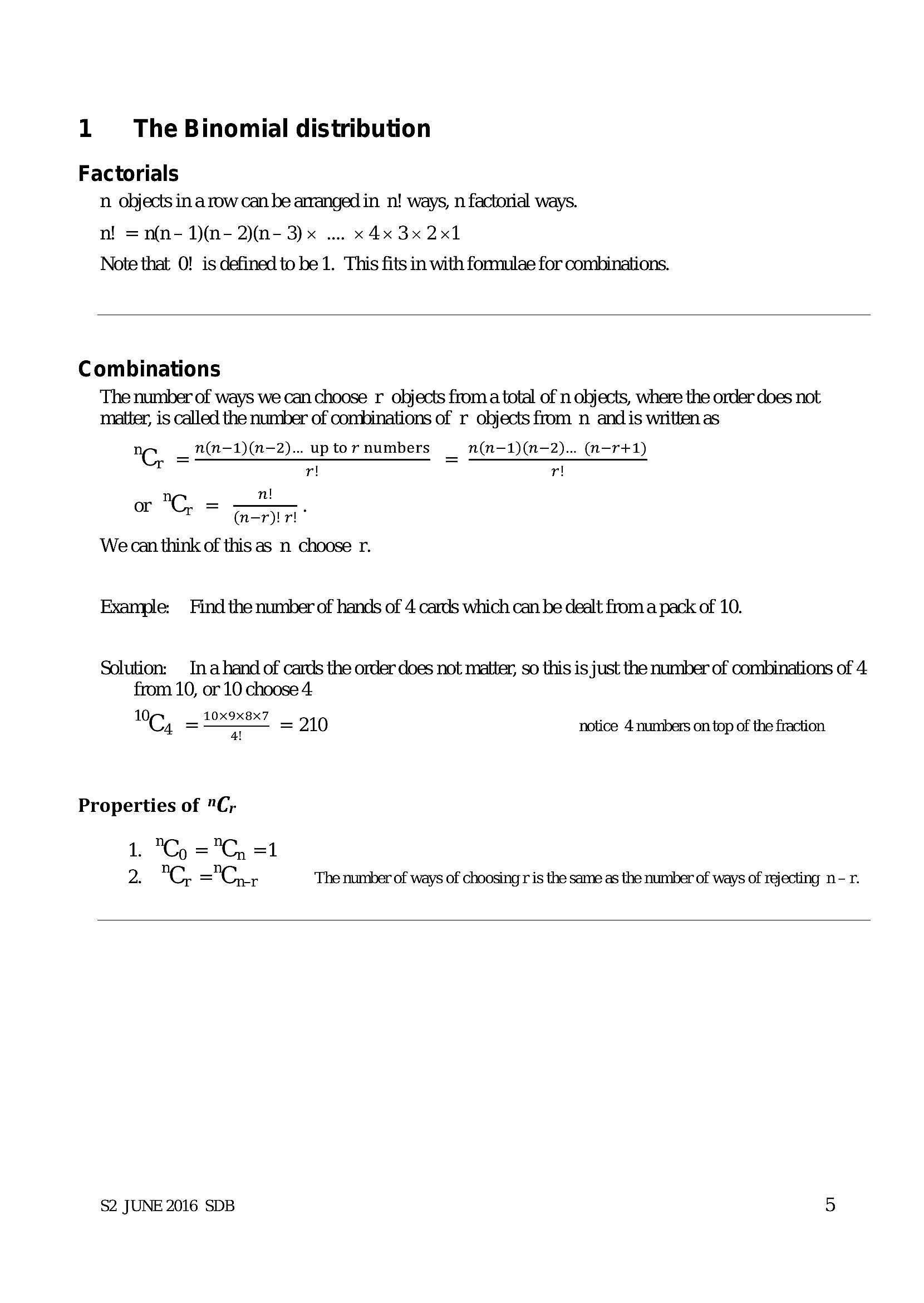
1 = The Binomial distributionFactorials
n objects ina row can be arranged in n! ways, n factorial ways.
=n(n- 1)(n- 2)(n- 3)x 1... x 4x 3x 2x1
Note that 0! is defined to be 1. This fits in with formulae for combinations.
Combinations
The number of ways we can choose r objects froma total of n objects, where the order does not
matter, is called the number of combinations of r objects from n and is written as
n(n—-1)(n—2)... up to 7 numbers n(n-1)(n—2)... (n—r+1)
"C, oS rr
or "C, =
We can think of this as n choose r.
(n- a ri?
Example: Find the number of hands of 4 cards which can be dealt from a pack of 10.
Solution: In ahand of cards the order does not matter, so this is just the number of combinations of 4
from 10, or 10 choose 4
C, ora“ = 210 notice 4 numbers on top of the fraction
Properties of "C;
1. "Cy ="C, =1
2. "C, ="Cr The number of ways of choosing r is the same as the number of ways of rejecting n- r.
$2 JUNE 2016 SDB 5
---
Page 8
Extracted Text
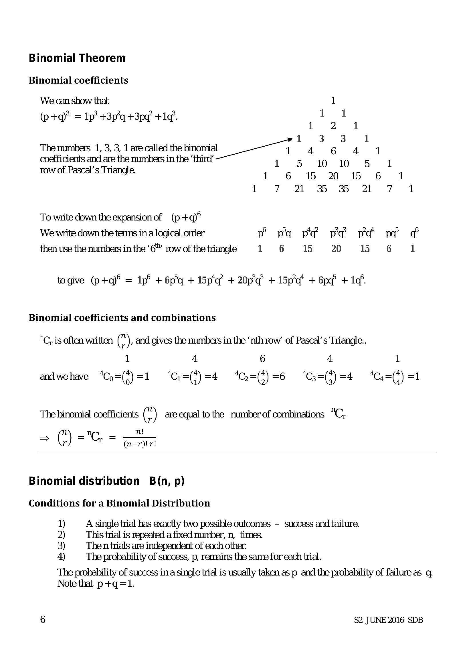
Binomial TheoremBinomial coefficients
‘We can show that 1
(p+q)? = Ip’ +3p’q +3pe" +1¢°.
1 3. 3 1
The numbers 1, 3, 3, 1 arecalledthebinomial 4 64 1
coefficients and are the numbers in the ‘third’
row of Pascal’s Triangle. 1 6 15 2 15 6 1
To write down the expansion of (p +q)°
We write down the tems in a logical order P pa po pa po pe @
then use the numbers in the ‘6”” row of the triangle 1 6 15 20 15 6 1
togive (p+q)° = 1p° + 6p + 15p'¢? + 20p’g? + 15p’q* + 6pg? + Id°.
Binomial coefficients and combinations
°C, is often written (), and gives the numbers in the ‘nth row of Pascal’s Triangle.
1 4 6 4 1
andwehave *Co=(4)=1 “Ci=(f)=4 “G=({)=6 “Ca=()=4 4a =(f) =1
The binomial coefficients (") are equal to the number of combinations "Cy
20) ==
(n-r)! r!
Binomial distribution B(n, p)
Conditions for a Binomial Distribution
1) A single trial has exactly two possible outcomes - success and failure.
2) This trial is repeated a fixed number, n, times.
3) The n trials are independent of each other.
4) The probability of success, p, remains the same for each trial.
The probability of success in a single trial is usually taken as p and the probability of failure as q.
Note that p+q=1.
6 $2 JUNE 2016 SDB
---
Page 9
Extracted Text
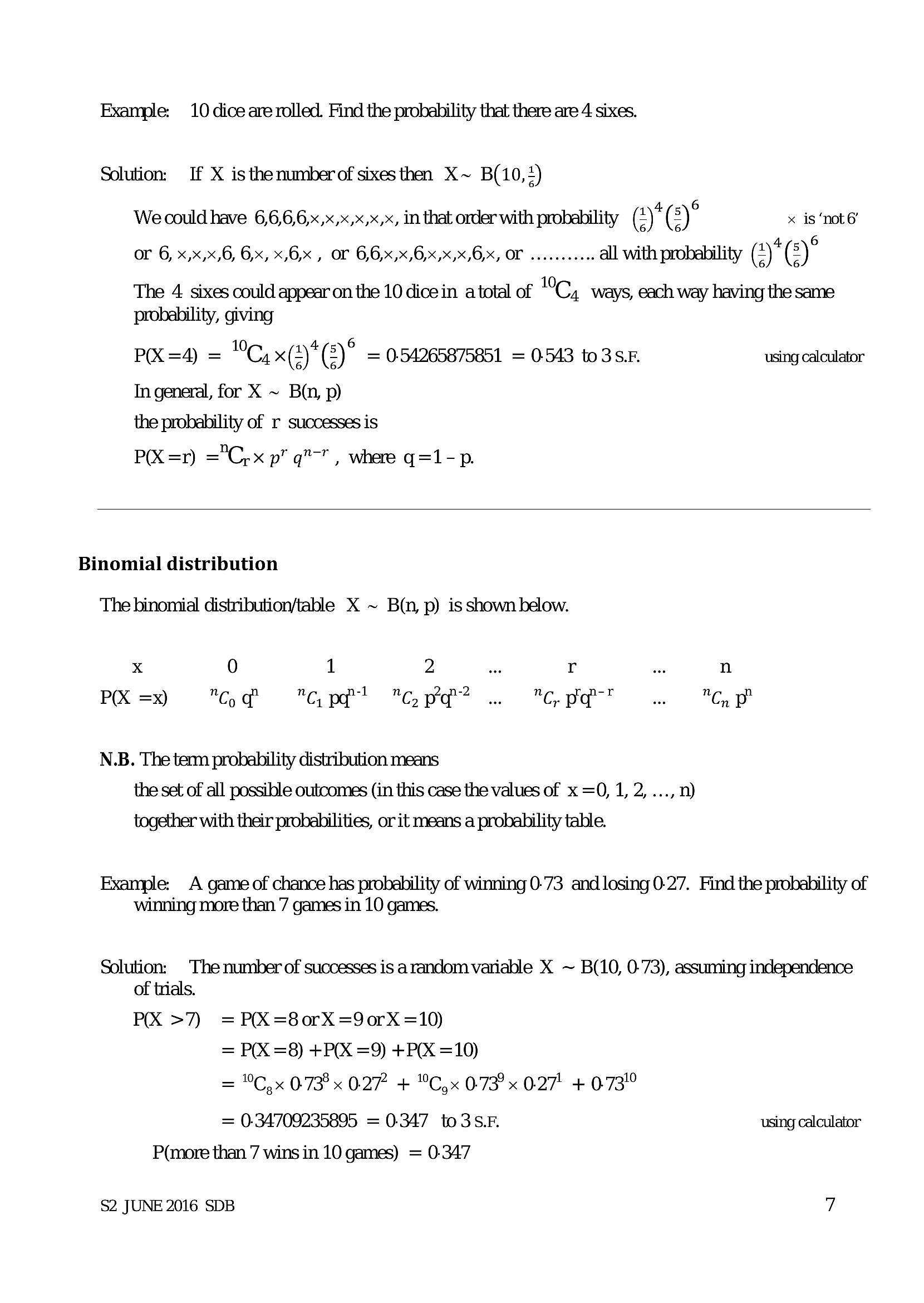
Example: 10 dice are rolled. Find the probability that there are 4 sixes.Solution: If X isthenumber of sixesthen X~ B(10,+)
We could have 6,6,6,6x,x,x,x,x,x, in that order with probability (2)*(2)° x is ‘note
OF 6, xx,x,6, 6%, x6, OF 6,6%)/6%) 6%) OF sees all with probability (2)*(8)°
The 4 sixes could appear on the 10 dice in a total of C, ways, each way having the same
probahility, giving
P(X =4) = "Cyx(2)*(2)° = 054265875851 = 0543 to3sF. using calculator
In general, for X ~ Bin, p)
the probability of r successes is
P(X=nr) ="C,x p' q”™" , where q=1-p.
Binomial distribution
The binomial distribution/table X ~ B(n, p) is shown below.
x 0 1 2 we r we n
P& =x) "Gq "Cpa? "pd? .. "pot. "CP
N.B. The tem probability distribution means
the set of all possible outcomes (in this case the values of x =0, 1, 2, ..., n)
together with their probabilities, or it means a probability table.
Example: A game of chance has probability of winning 0-73 and losing 0-27. Find the probability of
winning more than 7 games in 10 games.
Solution: The number of successes is arandom variable X ~ B(10, 0-73), assuming independence
of trials.
PX >7) = P(X =8o0rxX =9orxX =10)
= P(X =8) +P(X =9) +P(X =10)
= °C,x 073° x 0.27 + °Cyx 0-73? x 0.27' + 073°
= 034709235895 = 0347 to3s.F. using calculator
P(more than 7 wins in 10 games) = 0-347
$2 JUNE 2016 SDB 7
---
Page 10
Extracted Text
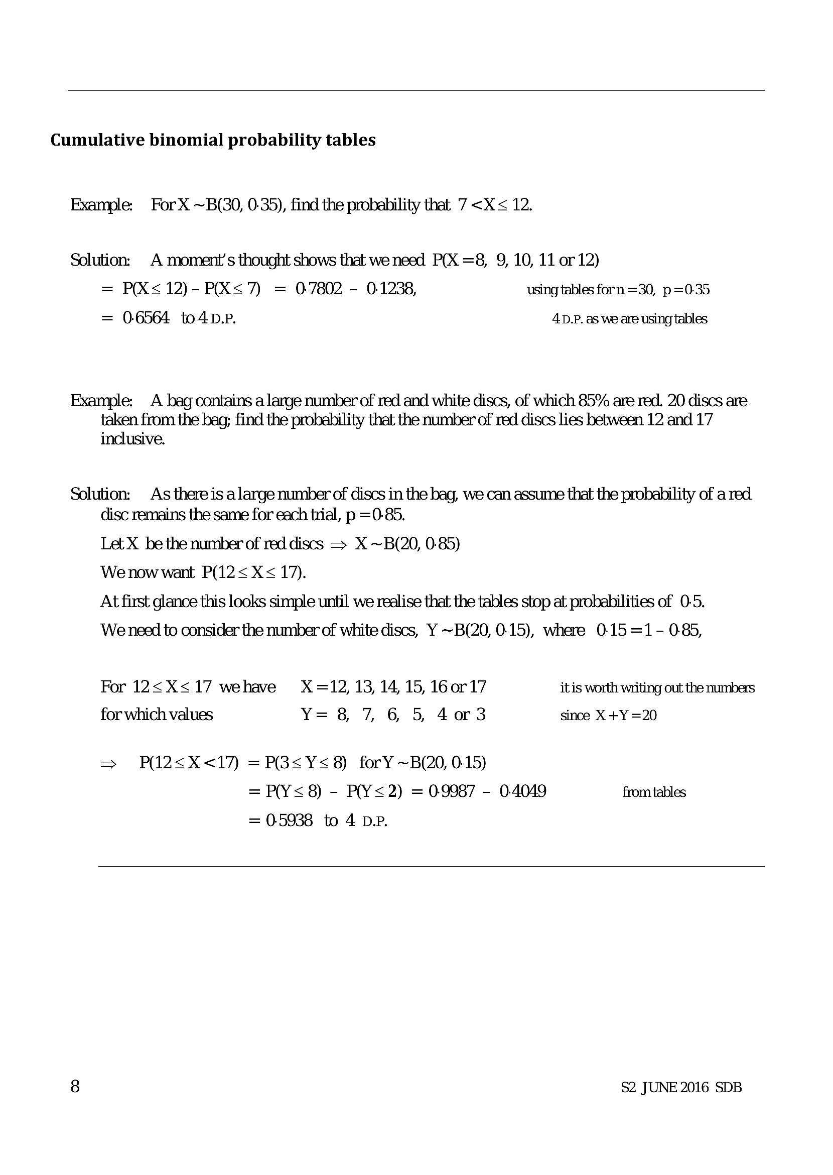
Cumulative binomial probability tablesExample: For X ~B(30, 0-35), find the probability that 7 <X< 12.
Solution: A moment’s thought shows that we need P(X =8, 9, 10, 11 or 12)
= PX<12)-P(X<7) = 07802 - 01238, using tables forn =30, p=0.35
= 06564 to4D-P. 4D.P. as we are using tables
Example: A bag contains a large number of red and white discs, of which 85% are red. 20 discs are
taken from the bag; find the probability that the number of red discs lies between 12 and 17
inclusive.
Solution: As there is alarge number of discs in the bag, we can assume that the probability of a red
disc remains the same for each tial, p =0-85.
Let X be the number of red discs > X ~B(20, 0-85)
We now want P(12< X< 17).
At first glance this looks simple until we realise that the tables stop at probabilities of 0-5.
We need to consider the number of white discs, Y ~B(20, 0-15), where 0-15 =1- 085,
For 12<X<17 wehave X=12,13 14,15, 160r17 itis worth writing out the numbers
for which values Y=8 7, 6 5, 4or3 since X +Y =20
=> P12<X<17) =P(3<Y<8) forY ~B(20, 0-15)
= P(Y<8) - P(Y<2) = 09987 - 0.4049 from tables
= 05938 to 4 DP.
8 $2 JUNE 2016 SDB
---
Page 11
Extracted Text
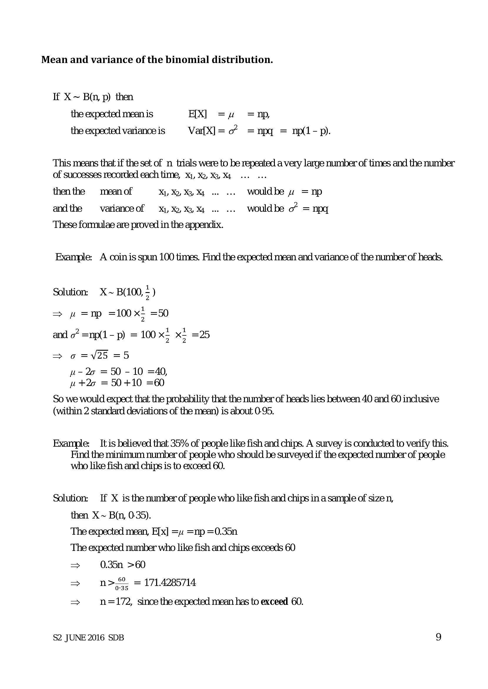
Mean and variance of the binomial distribution.If X ~ By, p) then
the expected mean is EX) =u =np,
the expected varianceis = Vaf{X]= 07 =npg = np(1-p).
This means that if the set of n trials were to be repeated a very large number of times and the number
of successes recorded each time, X1, X2, X3, Xa
thenthe meanof X1, Xy, XX... ... Wouldbe wz =np
andthe varianceof x1, %,%3,% ... ... wouldbe o* = npg
These formulae are proved in the appendix.
Example: A coinis spun 100 times. Find the expected mean and variance of the number of heads.
Solution. X~ B(100, ; )
a =np =100 x; =50
and o” =np(1-p) = 100 x5 x> =25
> ¢6 =V25 =5
u- 2s =50-10 =40,
u+2o =50+10 =60
So we would expect that the probability that the number of heads lies between 40 and 60 inclusive
(within 2 standard deviations of the mean) is about 0-95.
Example: Itis believed that 35% of people like fish and chips. A survey is conducted to verify this.
Find the minimum number of people who should be surveyed if the expected number of people
who like fish and chips is to exceed 60.
Solution: If X is the numberof people who like fish and chips in a sample of size n,
then X~ B(n, 0-35).
The expected mean, E[x] = =np =0.35n
The expected number who like fish and chips exceeds 60
> 0.35n >60
> n> = 171.4285714
> n=172, since the expected mean has to exceed 60.
$2 JUNE 2016 SDB 9
---
Page 12
Extracted Text
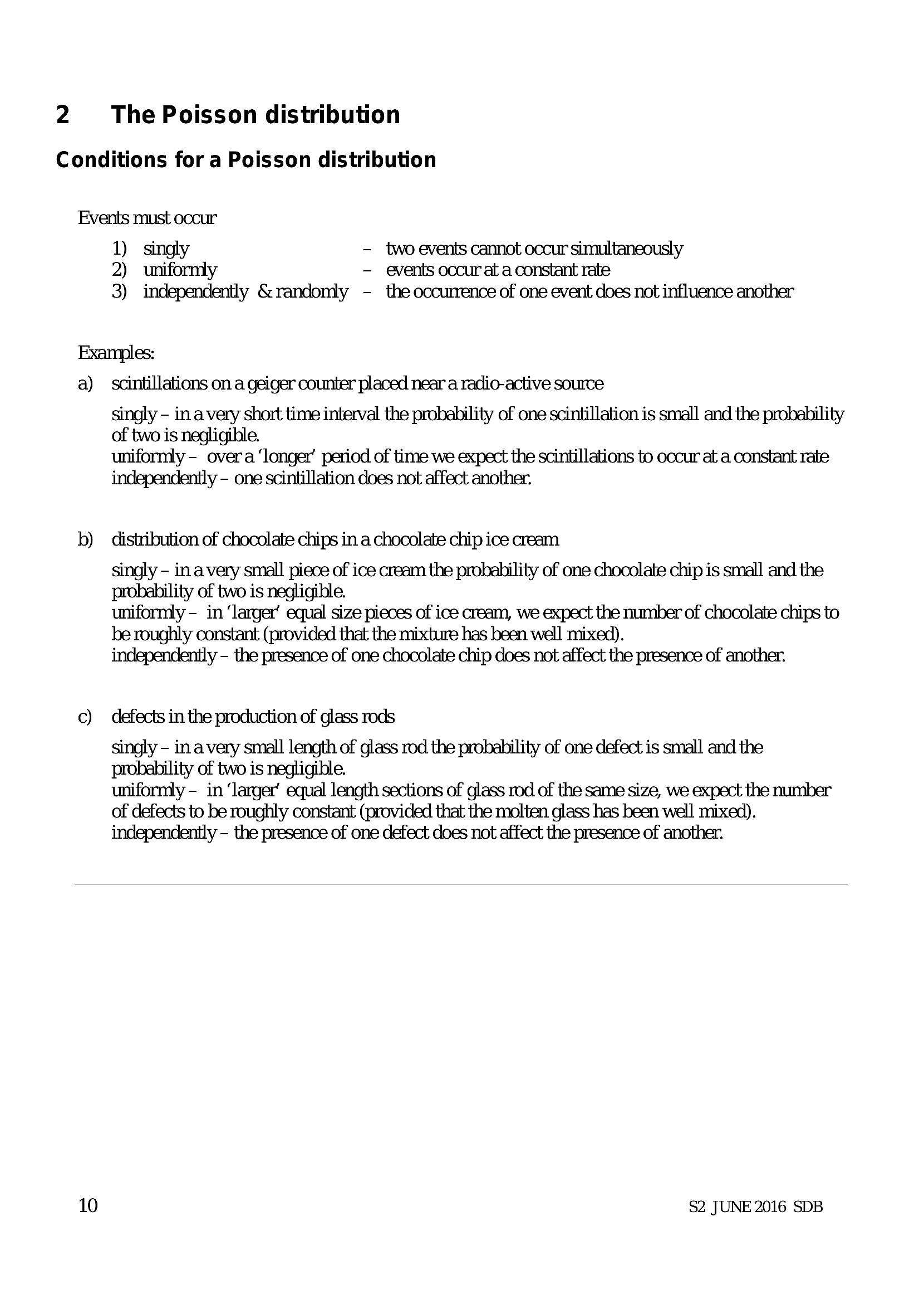
2The Poisson distribution
Conditions for a Poisson distribution
Events must occur
1) singly - two events cannot occur simultaneously
2) uniformly — events occur at a constant rate
3) independently &randomly - the occurrence of one event does not influence another
Examples:
a)
b)
Q
scintillations on a geiger counter placed near a radio-active source
singly - in avery short time interval the probability of one scintillation is small and the probability
of two is negligible.
uniformly- overa ‘longer’ period of time we expect the scintillations to occur at a constant rate
independently - one scintillation does not affect another.
distribution of chocolate chips in a chocolate chip ice cream
singly - in avery small piece of ice cream the probability of one chocolate chip is small and the
probability of two is negligible.
uniformly - in ‘larger’ equal size pieces of ice cream, we expect the number of chocolate chips to
be roughly constant (provided that the mixture has been well mixed).
independently - the presence of one chocolate chip does not affect the presence of another.
defects in the production of glass rods
singly - in avery small length of glass rod the probability of one defect is small and the
probability of two is negligible.
uniformly - in ‘larger’ equal length sections of glass rod of the same size, we expect the number
of defects to be roughly constant (provided that the molten glass has been well mixed).
independently - the presence of one defect does not affect the presence of another.
10
$2 JUNE 2016 SDB
---
Page 13
Extracted Text
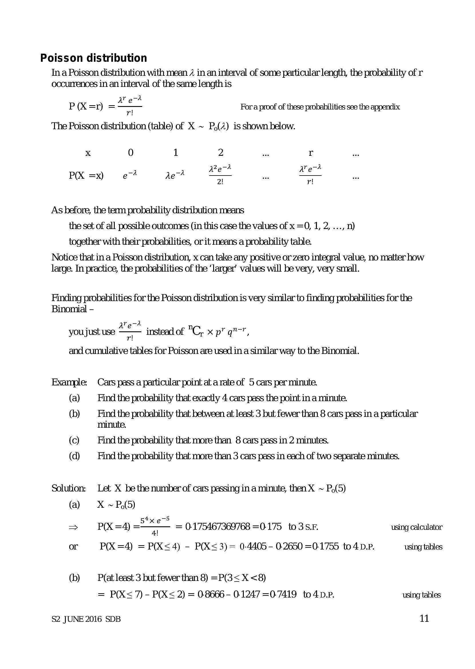
Poisson distribution Ina Poisson distribution with mean / in an interval of some particular length, the probability of r occurrences in an interval of the same length isav eA
r!|
The Poisson distribution (table) of X ~ P,(A) is shown below.
P(X=nr) =
For a proof of these probabilities see the appendix
x 0 1 2 we r
22 A a A
P(X =x) e774 de~* ° wn °
2! r!
As before, the term probability distribution means
the set of all possible outcomes (in this case the values of x =0, 1, 2, ..., n)
together with their probabilities, or it means a probability table.
Notice that in a Poisson distribution, x can take any positive or zero integral value, no matter how
large. In practice, the probabilities of the ‘larger’ values will be very, very small.
Finding probabilities for the Poisson distribution is very similar to finding probabilities for the
Binomial -
are-A
you just use — instead of "C, x p™ q”",
and cumulative tables for Poisson are used in a similar way to the Binomial.
Example: Cars pass a particular point at a rate of 5 cars per minute.
(a) Find the probability that exactly 4 cars pass the point in a minute.
(b) — Find the probability that between at least 3 but fewer than 8 cars pass in a particular
minute.
(c) Find the probability that more than 8 cars pass in 2 minutes.
(d) Find the probability that more than 3 cars pass in each of two separate minutes.
Solution: Let X be the number of cars passing in a minute, then X ~ P,(5)
(a) X~P,(5)
4 -5
P(X =4) = = 0:175467369768 =0175 to3SF. using calculator
or = P(X =4) = P(X<4) - P(X<3)= 0-4405- 02650 =0-1755 to4 DP. using tables
(b) — P(at least 3 but fewer than 8) =P(3< X <8)
= P(XX< 7) - P(X< 2) = 0.8666 - 0:1247=0-7419 to4D.P. using tables
$2 JUNE 2016 SDB 11
---
Page 14
Extracted Text
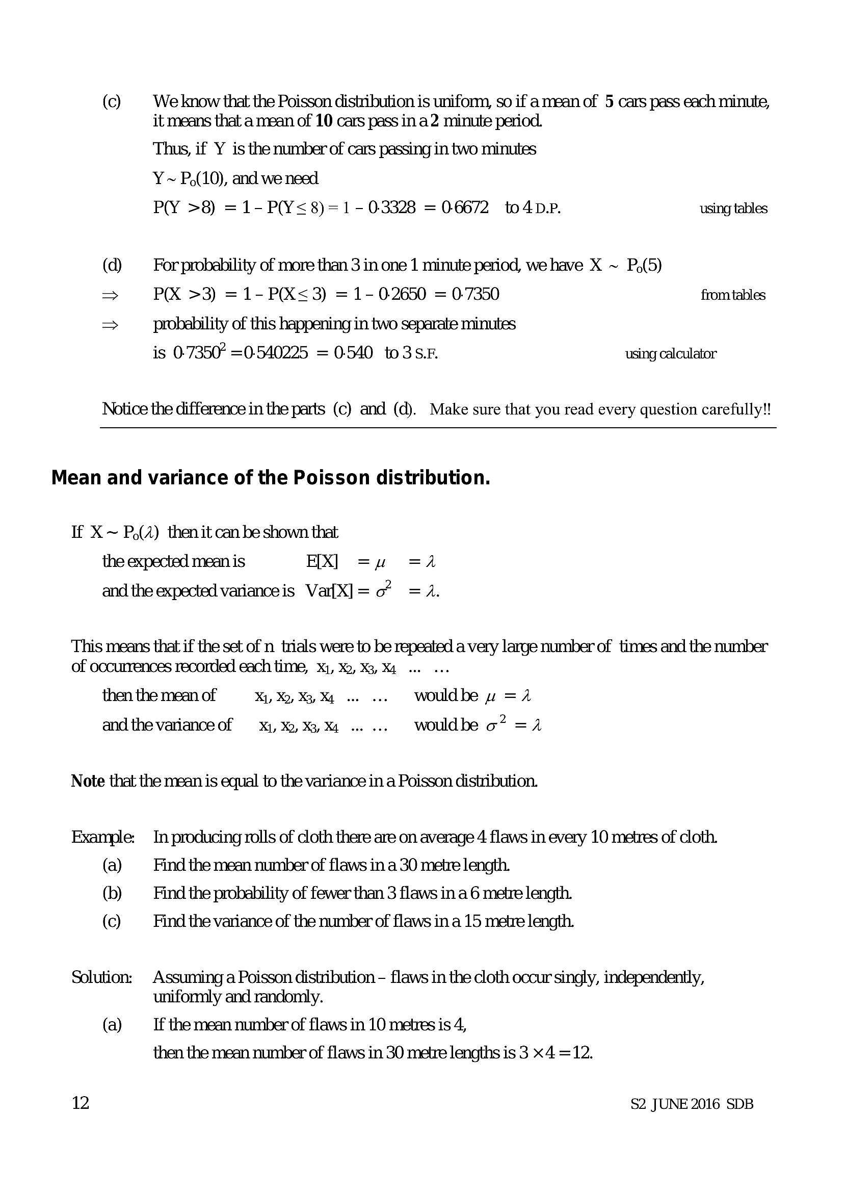
(c) We know that the Poisson distribution is uniform, so if a mean of 5 cars pass each minute, it means that a mean of 10 cars pass in a2 minute period.Thus, if Y is the number of cars passing in two minutes
Y ~ P,(10), and we need
PY >8) =1- P(Y<8)=1 - 03328 =06672 to4D-P. using tables
(d) For probability of more than 3 in one 1 minute period, we have X ~ P,(5)
=> P(X >3) = 1-P(K<3) =1- 02650 = 07350 from tables
> probability of this happening in two separate minutes
is 0-7350° =0-540225 =0-40 to3sS.F using calculator
Notice the difference in the parts (c) and (d). Make sure that you read every question carefully!
Mean and variance of the Poisson distribution.
If X ~ P,(A) then it can be shown that
the expected mean is EX] =u =a
and the expected varianceis Vaf{X]= 07 =A.
This means that if the set of n trials were to be repeated a very large number of times and the number
of occurrences recorded each time, X41, X2, X3, X4 oo.
then the mean of X1, Xy, XB, Xe .. ... wouldbe w =1
andthe varianceof x1, %),%3%4 ...... wouldbe o? =
Note that the mean is equal to the variance in a Poisson distribution.
Example: In producing rolls of cloth there are on average 4 flaws in every 10 metres of cloth.
(a) Find the mean number of flaws in a 30 metre length.
(b) Find the probability of fewer than 3 flaws in a 6 metre length.
(co) Find the variance of the number of flaws in a 15 metre length.
Solution: Assuming a Poisson distribution - flaws in the cloth occur singly, independently,
unifomnly and randomly.
(a) If the mean number of flaws in 10 metres is 4,
then the mean number of flaws in 30 metre lengths is 3 x4 =12.
12 $2 JUNE 2016 SDB
---
Page 15
Extracted Text
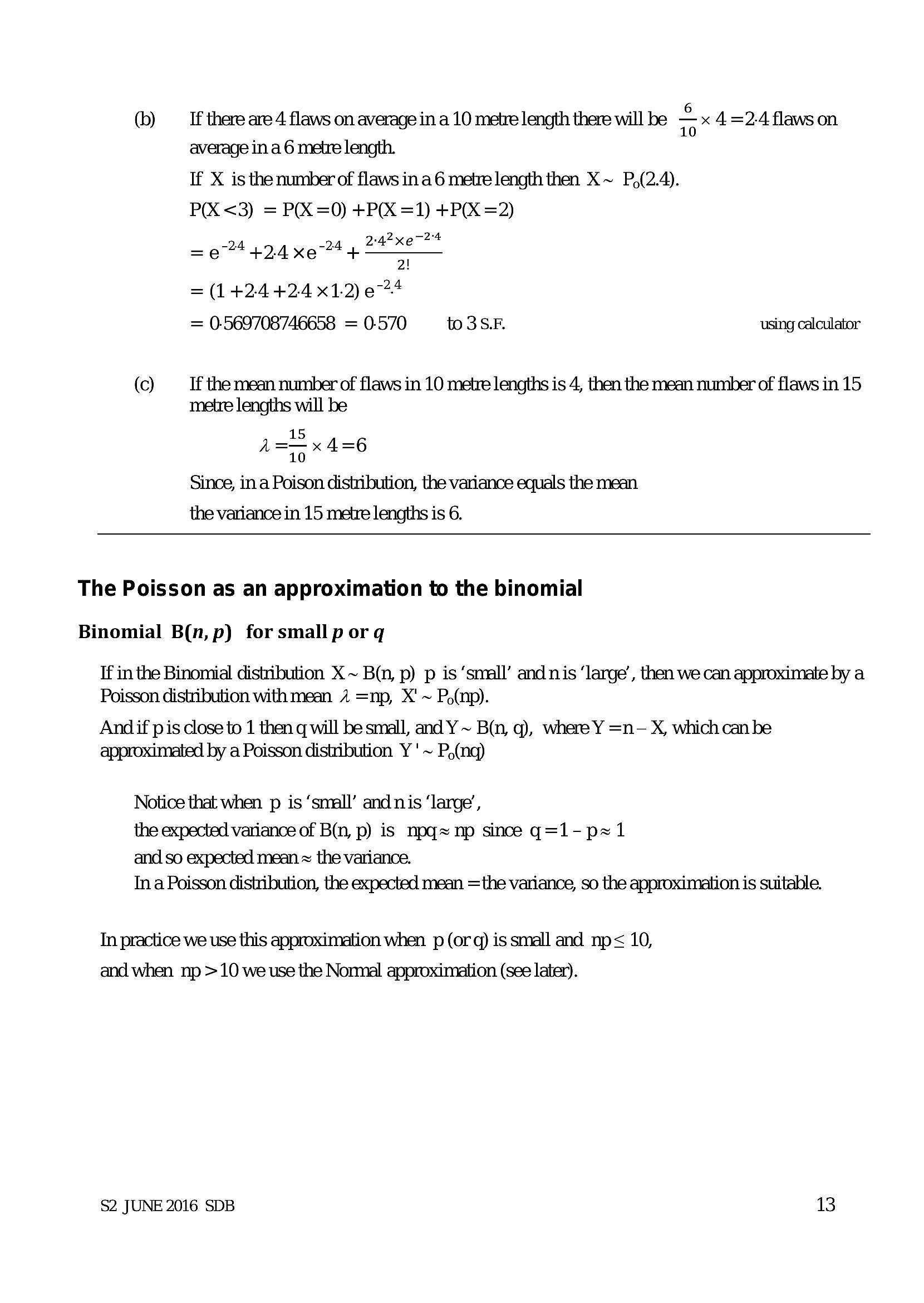
(b) If there are 4 flaws on average in a 10 metre length there will be = x 4 =2-4 flaws on average in a 6 metre length. If X is the number of flaws ina 6 metre length then X~ P,(2.4). P(X <3) = P(X =0) + P(X =1) + P(X =2) 242xe72'4 2! = (1424424 x1.2)e%4 = 0-569708746658 = 0-570 to3SF. using calculator=e 4424 xe 74 +
(co) If the mean number of flaws in 10 metre lengths is 4, then the mean number of flaws in 15
metre lengths will be
A= x 4=6
10
Since, in a Poison distribution, the variance equals the mean
the variance in 15 metre lengths is 6.
The Poisson as an approximation to the binomial
Binomial B(n, p) for small p or q
If in the Binomial distribution X ~ Bin, p) p is ‘small’ and nis ‘large’, then we can approximate by a
Poisson distribution with mean 1 =np, X' ~ P,(np).
And if pis close to 1 then q will be small, and Y ~ B(n, q), where Y =n-— X, which can be
approximated by a Poisson distribution Y '~ P,(nq)
Notice that when p is ‘small’ and nis ‘large’,
the expected variance of B(n, p) is npq~ np since q=1-px1
and so expected mean ~ the variance.
In a Poisson distribution, the expected mean =the variance, so the approximation is suitable.
In practice we use this approximation when p (or q) is small and np< 10,
and when np > 10 we use the Nomnal approximation (see later).
$2 JUNE 2016 SDB 13
---
Page 16
Extracted Text
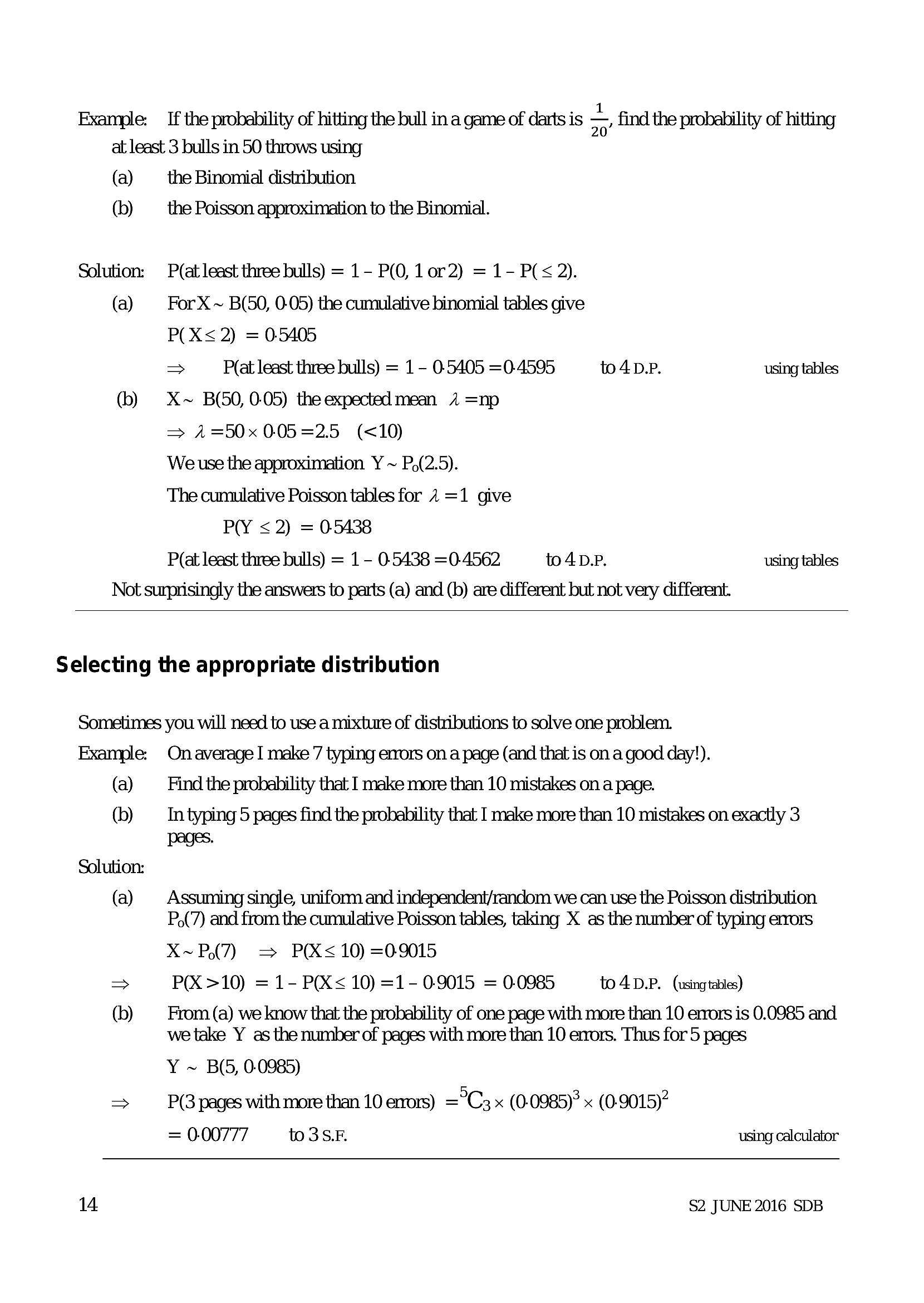
Example:If the probability of hitting the bull in a game of darts is =, find the probability of hitting
at least 3 bulls in 50 throws using
(a)
(b)
Solution:
(a)
(b)
the Binomial distribution
the Poisson approximation to the Binomial.
P(at least three bulls) = 1- P(0, 1or2) = 1- P(< 2).
For X ~ B(50, 0-05) the cumulative binomial tables give
P(X< 2) = 05405
> P(at least three bulls) = 1 - 05405 =0-4595 to4D.P. using tables
X~ B(50, 0-05) the expected mean 2 =np
=> 4=50x 005=2.5 (<10)
Weuse the approximation Y ~ P,(2.5).
The cumulative Poisson tables for 1 =1 give
PY < 2) = 05438
P(at least three bulls) = 1 - 0-5438 =0-4562 to4D.P. using tables
Not surprisingly the answers to parts (a) and (b) are different but not very different.
Selecting the appropriate distribution
Sometimes you will need to use a mixture of distributions to solve one problem.
Example:
(a)
(b)
Solution:
(a)
(b)
On average I make 7 typing emors on a page (and that is on a good day!).
Find the probability that I make more than 10 mistakes on a page.
In typing 5 pages find the probability that I make more than 10 mistakes on exactly 3
pages.
Assuming single, uniform and independent/random we can use the Poisson distribution
P,(7) and from the cumulative Poisson tables, taking X as the number of typing emors
X~P(7) = P(X< 10) =09015
P(X >10) = 1- P(X< 10) =1- 0.9015 = 0.0985 to4D.P. (using tables)
From (a) we know that the probability of one page with more than 10 errors is 0.0985 and
we take Y as the number of pages with more than 10 errors. Thus for 5 pages
Y ~ B(5, 0.0985)
P(3 pages with more than 10 errors) ="C3 x (0- 0985)" x (0- 9015)"
= 0.00777 to3S.F using calculator
14
$2 JUNE 2016 SDB
---
Page 17
Extracted Text
3 Continuous random variablesProbability density functions
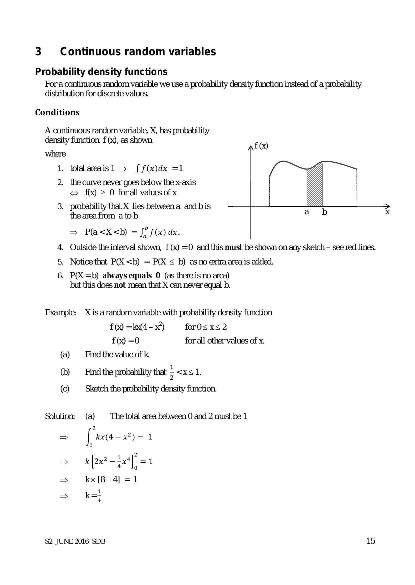
For a continuous random variable we use a probability density function instead of a probability
distribution for discrete values.
Conditions
A continuous random variahle, X, has probability
density function f (x), as shown
where
1. totalaraisl > ff(x)dx =1
2. the curve never goes below the x-axis
<= f(x) = 0 forall values ofx
3. probability that X lies betweena and bis
the area from a to b
=> P(a<X<b) = fo F@) dx.
4. Outside the interval shown, f(x) =O and this must be shown on any sketch - see red lines.
5. Notice that P(X <b) = P(X < b) asno extraareais added.
6. P(X =b) always equals 0 (as thereis no area)
but this does not mean that X can never equal b.
Example: X is arandom variable with probability density function
f(x) =kk(4-x) — for0<x<2
f(x) =0 for all other values of x.
(a) ‘Find the value of k.
(b) Find the probability that <x<1.
(c) Sketch the probability density function.
Solution: (a) The total area between 0 and 2 must be 1
2
> I kx(4—x7)=1
0
k [2x2 —x4]° =1
> [2x 74% I, =
> kx [8-4] =1
$2 JUNE 2016 SDB 15
---
Page 18
Extracted Text
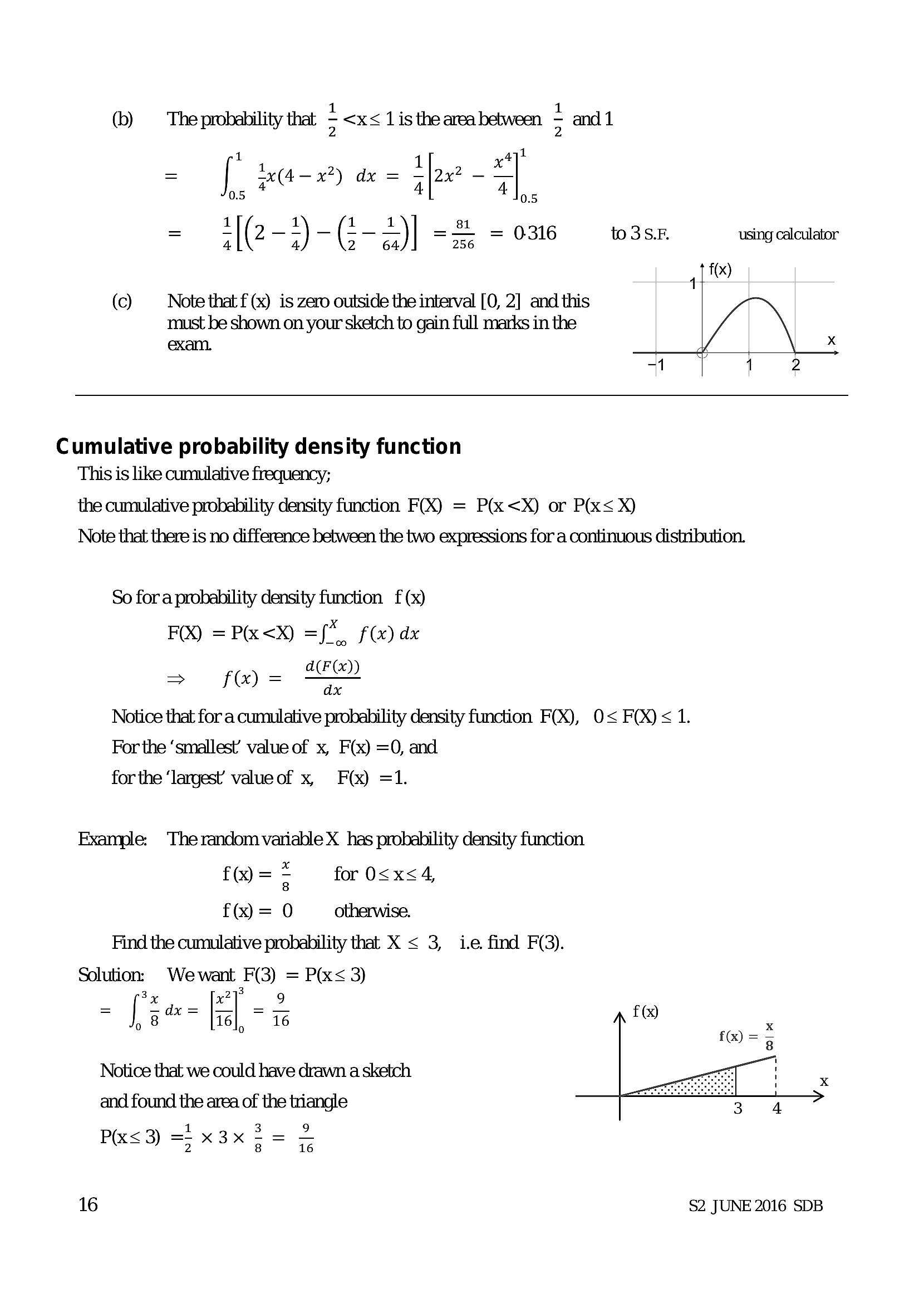
(b) The probability that *= | ax(4— x?) dx = sox" - a
0.5 4 4 N55
= ‘(2 _ *) - G - ~)| =" = 0316 to3SF. using calculator
(c) Note that f (x) is zero outside the interval [0, 2] and this
must be shown on your sketch to gain full marks in the
exam.
Cumulative probability density function
This is like cumulative frequency;
the cumulative probability density function FX) = P(x<X) or P(x< X)
Note that there is no difference between the two expressions for a continuous distribution.
So fora probability density function f (x)
FO) =P(x<X) ={", f(x) dx
a(F
= fo=
Notice that for a cumulative probability density function FX), 0< FOX) < 1.
For the ‘smallest’ value of x, F(x) =O, and
for the ‘largest’ value of x, F(x) =1.
Example: The random variable X has probability density function
f@==> for 0<x<4,
f= 0 otherwise.
Find the cumulative probability that X < 3, ie find F(9).
Solution: Wewant F(3) = P(x< 3)
- [ia- |e] -2
, 8° | 16), ~ 16
Notice that we could have drawn a sketch
and found the area of the triangle
P(x< 3) =; x3x - = =
16
$2 JUNE 2016 SDB
---
Page 19
Extracted Text
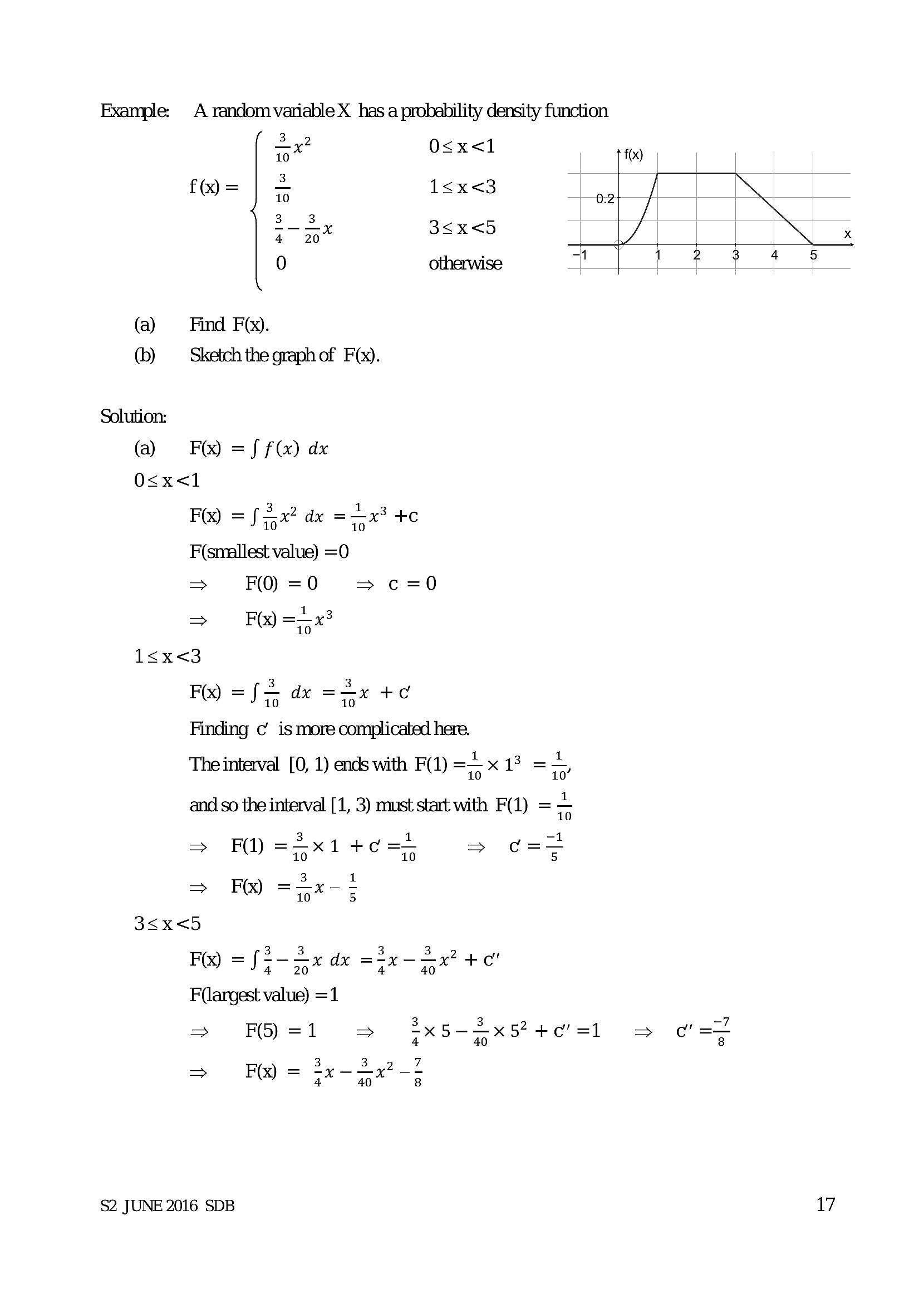
Example: A random variable X has a probability density function32 O<x<1
10
f@= | = 1<x<3
3_3,y 3<x<5
4 20
0 otherwise
(b) — Sketch the graph of F(x).
Solution:
(a) FQ) =f f(x) dx
O<x<l
FO) = fax? dx =—x? +c
F(smallest value) =0
> F(O) =0 > c=0
> FR =5x3
1<x<3
F(x) =f= dx =< x +c
Finding c’ is more complicated here.
The interval [0, 1) ends with F(1) == x 13 =<,
and so the interval [1, 3) must start with F(1) ==
3 1 -1
FI) = x1 +c => c=—
3 1
= FQ) =5x-=
3<x<5
F(X) = f2-sx dx =ix-Sx? +c"
F(argest value) =1
=> FS=1 = 3x5-Sxs4e'sl = oat
3 3 7
> F(X) = qx Qe 3
$2 JUNE 2016 SDB 17
---
Page 20
Extracted Text
>(b)
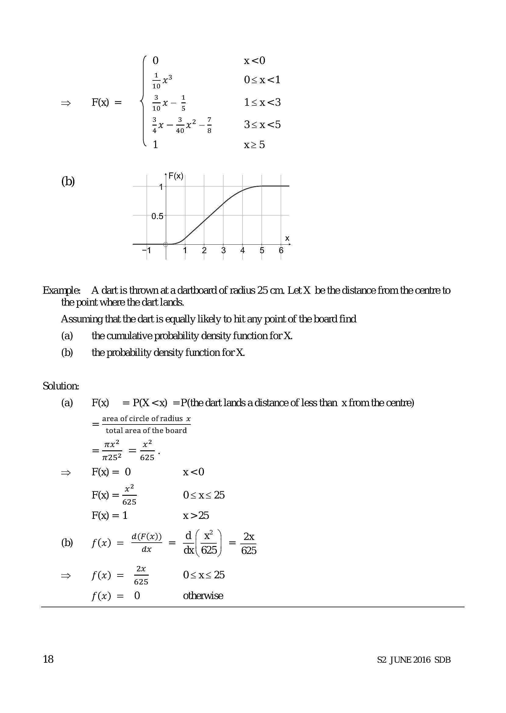
0) x<0
+x O<x<1
10
F(x) = =x 1<x<3
3y-3 42-2 3<x<5
4 8
1 x25
Example: A dart is thrown at a dartboard of radius 25 cm. Let X be the distance from the centre to
the point where the dart lands.
Assuming that the dart is equally likely to hit any point of the board find
the cumulative probability density function for X.
(a)
(b)
the probability density function for X.
Solution:
(a) FQ) = P(X <x) =P(the dart lands a distance of less than x from the centre)
__ area of circle of radius x
total area of the board
amet
“71252625 "
> F@) = 0 x<0
x2
Fx) = — O<x< 25
625
F@)=1 x>25
d(F(x)) d(x 2x
Db = = =
0) 10) = ax +5] 625
2x
> f(x) = o25 O<x<25
f@) = 0 otherwise
18 $2 JUNE 2016 SDB
---
Page 21
Extracted Text
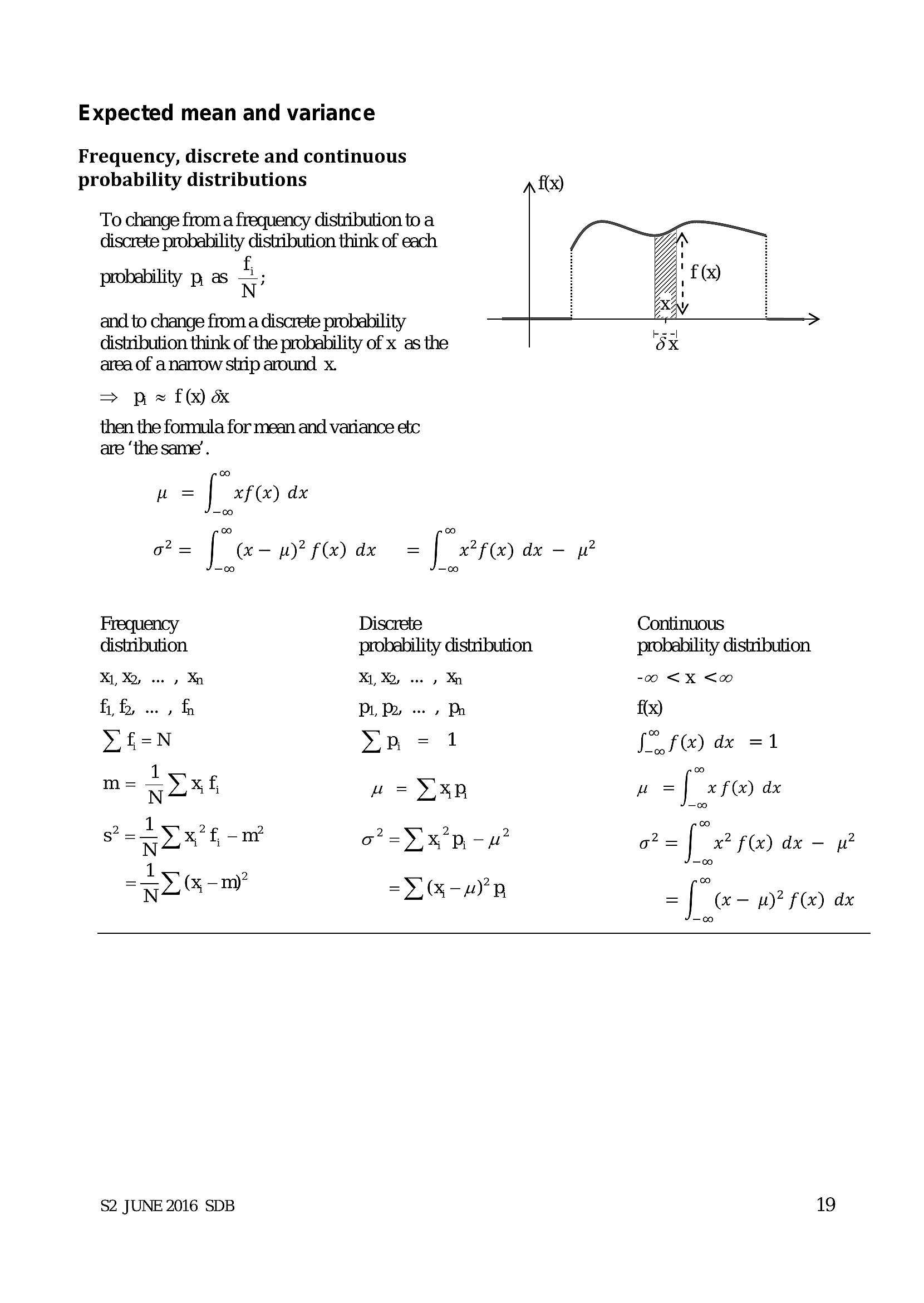
Expected mean and varianceFrequency, discrete and continuous
probability distributions f(x)
To change from a frequency distribution to a
discrete probability distribution think of each
probability p as a
a
XEN)
and to change from a discrete probability aN >
distribution think of the probability of x as the ‘5X
area of a narrow strip around x.
=> px f&) %K
then the formula for mean and variance etc
are ‘the same’.
Lu -| xf (x) dx
=f w-wsf@ar =f eed -
Frequency Discrete Continuous
distribution probability distribution probability distibution
X, Xa, .. » Mn XX, .. » Xn -00 <XK <0o
fib... fh Pi, Py -. » Ph f(x)
Yf=N Yp=1 [rf @) dx =1
1 foe)
m= 5x6 “w= >xD u =[ xf) dx
1 co
s= xf nr oF =x pu? ot = | x? f(x) dx — yw?
1 —oco
==>) (x -m? = -— u)* “
Nm X i AYP, =| (x - pw)? f(x) dx
$2 JUNE 2016 SDB 19
---
Page 22
Extracted Text
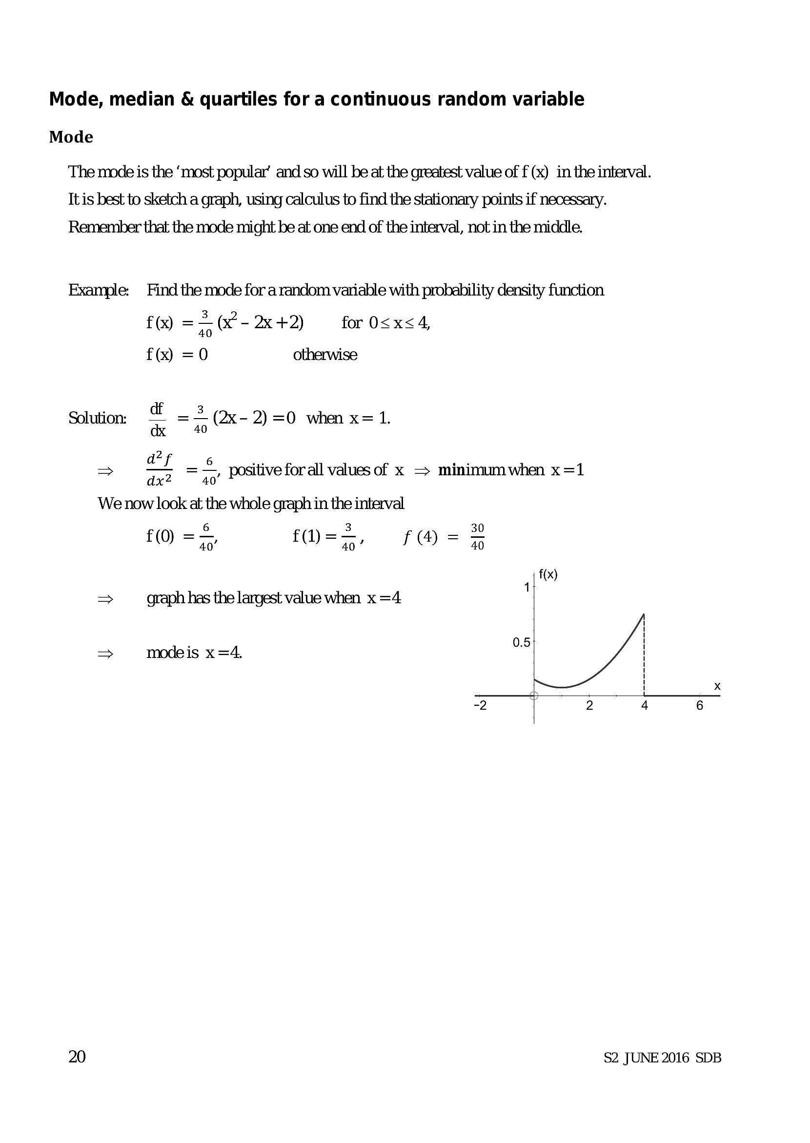
Mode, median & quartiles for a continuous random variable ModeThe mode is the ‘most popular’ and so will be at the greatest value of f (x) in the interval.
It is best to sketch a graph, using calculus to find the stationary points if necessary.
Remember that the mode might be at one end of the interval, not in the middle.
Example: Find the mode for a random variable with probability density function
f() == (-2x+2) for O<x<4,
f(x) =0 otherwise
. df 3
Solution. =— =— (2x-2)=0 when x= 1.
dx 40
af 6 «a: .
> 2 a0! positive for all values of x = minimum when x=1
We now look at the whole graph in the interval
6 3 30
£0) =>) fD=7) fHMA= A
f(x)
=> graph has the largest value when x =4 '
0.5
> modeis x =4,
1
iN)
iD)
Ne
o
20 $2 JUNE 2016 SDB
---
Page 23
Extracted Text
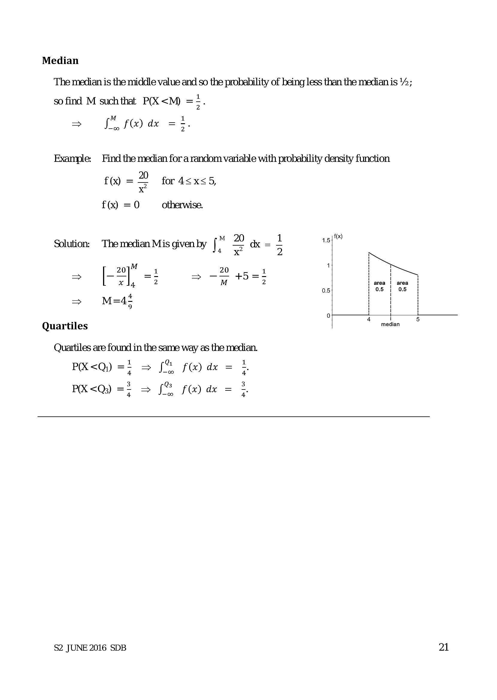
MedianThe median is the middle value and so the probahility of being less than the median is ¥2;
so find M suchthat P(X <M) =5.
> en f(x) dx = :.
Example: Find the median for a random variable with probability density function
f() = for 4<x<5,
x
f(x) =0 otherwise.
Solution: Themedian Mis givenby [" 22 dx
xX
M
20 1 20 1
> | xl, 2 > ay t83
=> M=4!
9
Quartiles
Quartiles are found in the same way as the median.
PR<Q) =5 => f% fi) dx = 5
PK <Q) =5 > JS fe) de = 2
1.5
0.5
or panne eee ee.
i
median
$2 JUNE 2016 SDB
21
---
Page 24
Extracted Text
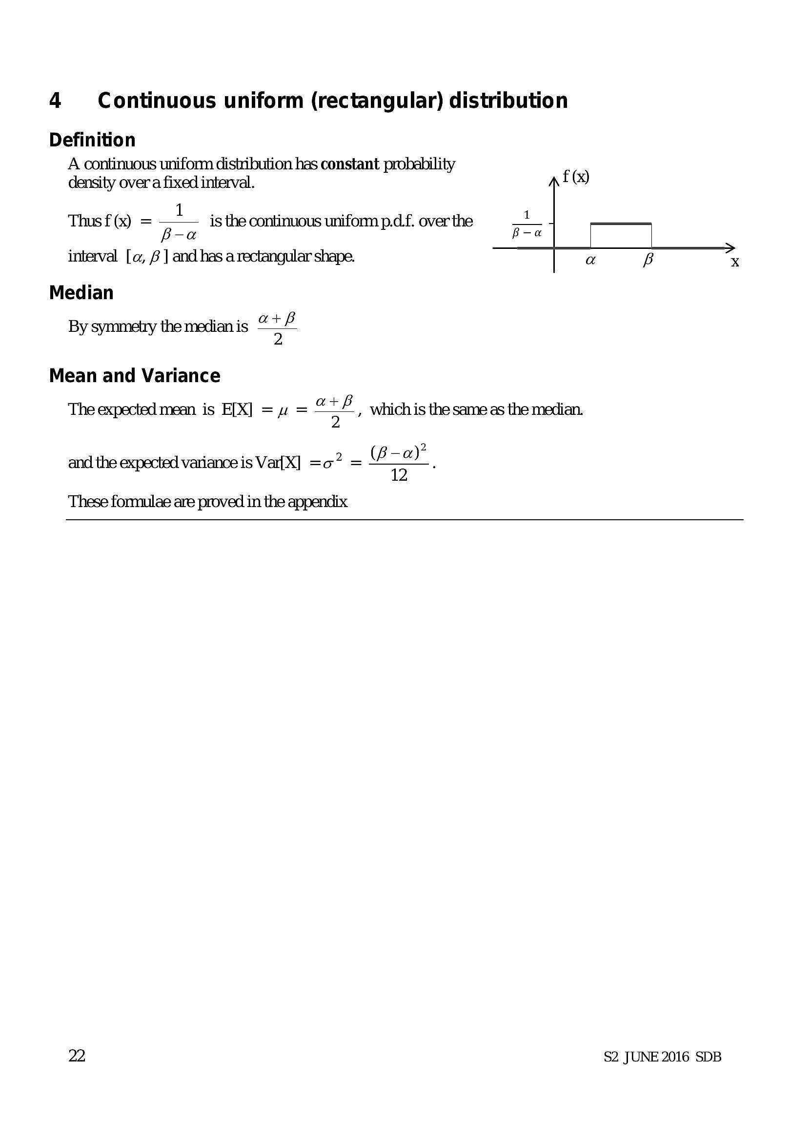
4 Continuous uniform (rectangular) distribution DefinitionA continuous uniform distribution has constant probability
density overa fixed interval. f(x)
Thus f(x) = is the continuous uniform p.d.f. over the
interval [a, £ ] and has a rectangular shape.
Median
By symmetry the median is ae
Mean and Variance
The expected mean is E[X] = uw = oF, which is the same as the median.
2
and the expected variance is Var{X] =o? = oa
These formulae are proved in the appendix
22 $2 JUNE 2016 SDB
---
Page 25
Extracted Text
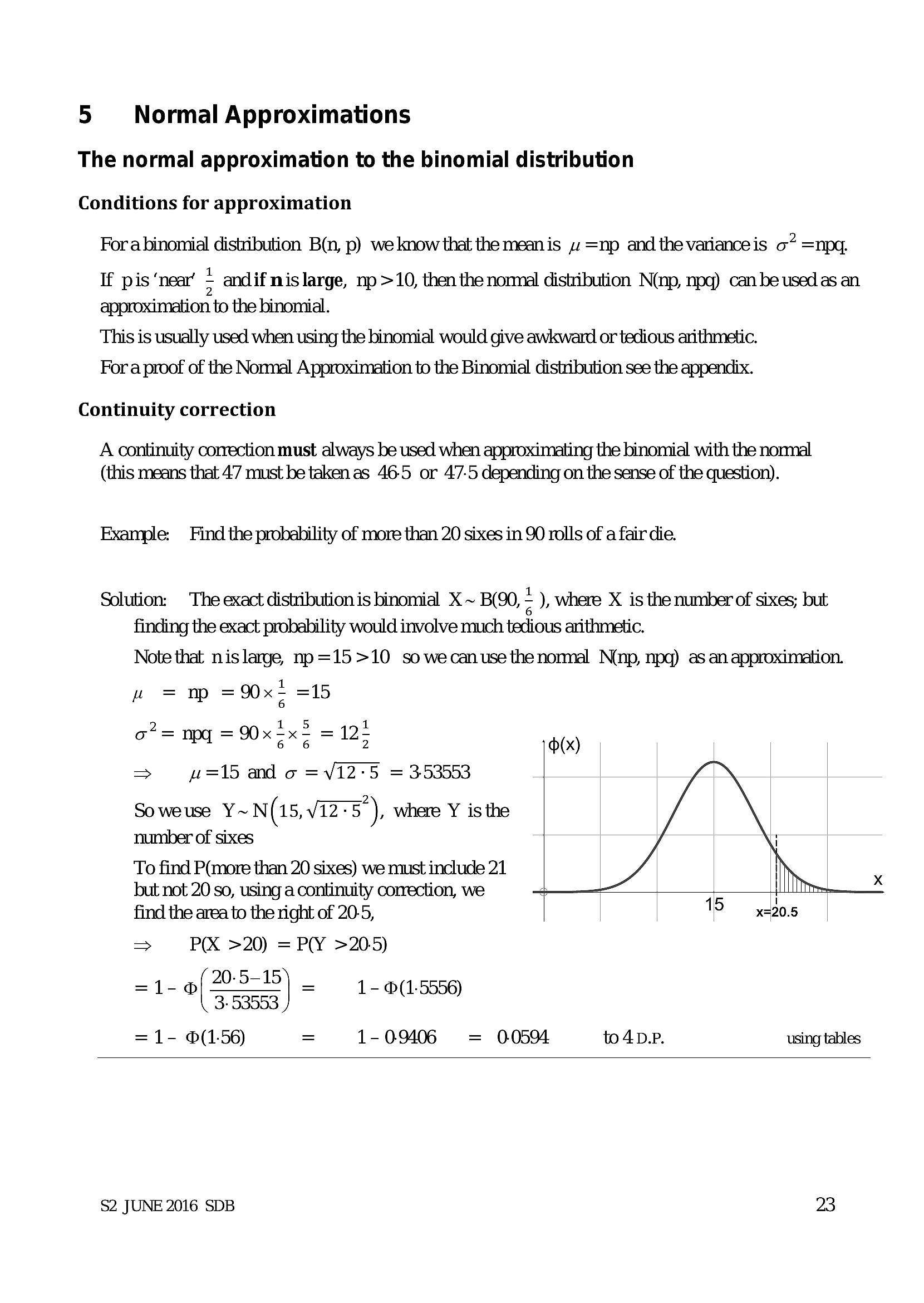
5 Normal Approximations The normal approximation to the binomial distribution Conditions for approximationForabinomial distribution B(n, p) we know that the mean is 4s =np and the varianceis o” =npq.
If pis ‘near’ ; andif nis large, np >10, then the normal distribution N(np, npq) can be used as an
approximation to the binomial.
This is usually used when using the binomial would give awkward or tedious arithmetic.
Fora proof of the Normal Approximation to the Binomial distribution see the appendix.
Continuity correction
A continuity correction must always be used when approximating the binomial with the normal
(this means that 47 must be taken as 46-5 or 47-5 depending on the sense of the question).
Example: Find the probability of more than 20 sixes in 90 rolls of a fair die.
Solution: The exact distribution is binomial X ~ B(90, = ), where X is the number of sixes; but
finding the exact probability would involve much tedious arithmetic.
Note that nislarge, np =15>10 so wecanuse the normal Nnp, npq) as an approximation.
we = mp =9x= =15
1.5
o* = npg = 90x 2x = = 12+
(x)
> w=15 and o =V12-5 =353553
Soweuse Y~N(15,vi2-5 ), where Y isthe
number of sixes
To find P(more than 20 sixes) we must include 21
but not 20 so, using a continuity correction, we
find the area to the right of 20-5,
=> PX >20) = PY >205)
-1- of M58
3- 53553
=1- (1.56) = 1-09406 = 00594 to4D.P. using tables
} = 1- @(1.-5556)
$2 JUNE 2016 SDB 23
---
Page 26
Extracted Text
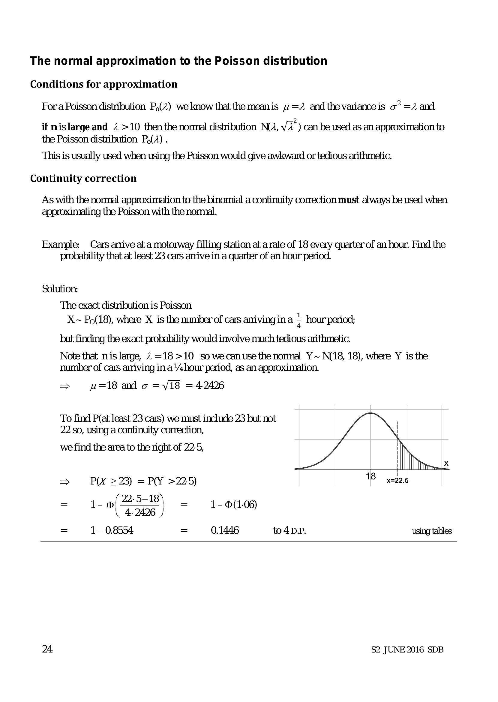
The normal approximation to the Poisson distribution Conditions for approximationFora Poisson distribution P,(2) we know that the meanis 4 =/ and the variance is o* =A and
if nislarge and 2 >10 then the normal distribution NA, V2) can be used as an approximation to
the Poisson distribution P,(/) .
This is usually used when using the Poisson would give awkward or tedious arithmetic.
Continuity correction
As with the normal approximation to the binomial a continuity correction must always be used when.
approximating the Poisson with the normal.
Example: Cars arrive at a motorway filling station at a rate of 18 every quarter of an hour. Find the
probability that at least 23 cars arive in a quarter of an hour period.
Solution:
The exact distribution is Poisson
X~ PQ(18), where X is the number of cars arriving ina ; hour period;
but finding the exact probability would involve much tedious arithmetic.
Note that nislarge, 7 =18>10 so wecanusethe normal Y~ N18, 18), where Y is the
number of cars amiving in a Yahour period, as an approximation.
> w=18 and o =V18 = 42426
To find P(at least 23 cars) we must include 23 but not
22 So, using a continuity correction, i
we find the area to the right of 22:5,
| xX
> PX >23) =P(Y >225) 18 y2225
= 1- 0 Ee | = 1-0(1.06
4. 2426
= 1-0.8554 = 01446 toApe. using tables
24 $2 JUNE 2016 SDB
---
Page 27
Extracted Text
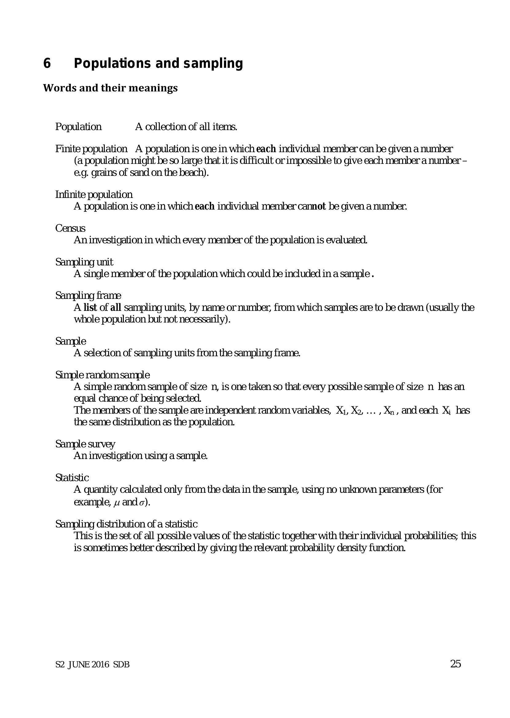
6 Populations and samplingWords and their meanings
Population A collection of all items.
Finite population A population is one in which each individual member can be given a number
(a population might be so large that it is difficult or impossible to give each member a number -
e.g. grains of sand on the beach).
Infinite population
A population is one in which each individual member cannot be given a number.
Census
An investigation in which every member of the population is evaluated.
Sampling unit
A single member of the population which could be included in a sample .
Sampling frame
A list of all sampling units, by name or number, from which samples are to be drawn (usually the
whole population but not necessarily).
e
A selection of sampling units from the sampling frame.
Simple randomsample
A simple random sample of size n, is one taken so that every possible sample of size n has an
equal chance of being selected.
The members of the sample are independent random variables, Xj, Xo, ... , Xn, and each X; has
the same distribution as the population.
Sample survey
An investigation using a sample.
Statistic
A quantity calculated only from the data in the sample, using no unknown parameters (for
example, ando).
Sampling distribution of a statistic
This is the set of all possible values of the statistic together with their individual probabilities; this
is sometimes better described by giving the relevant probability density function.
$2 JUNE 2016 SDB 25
---
Page 28
Extracted Text
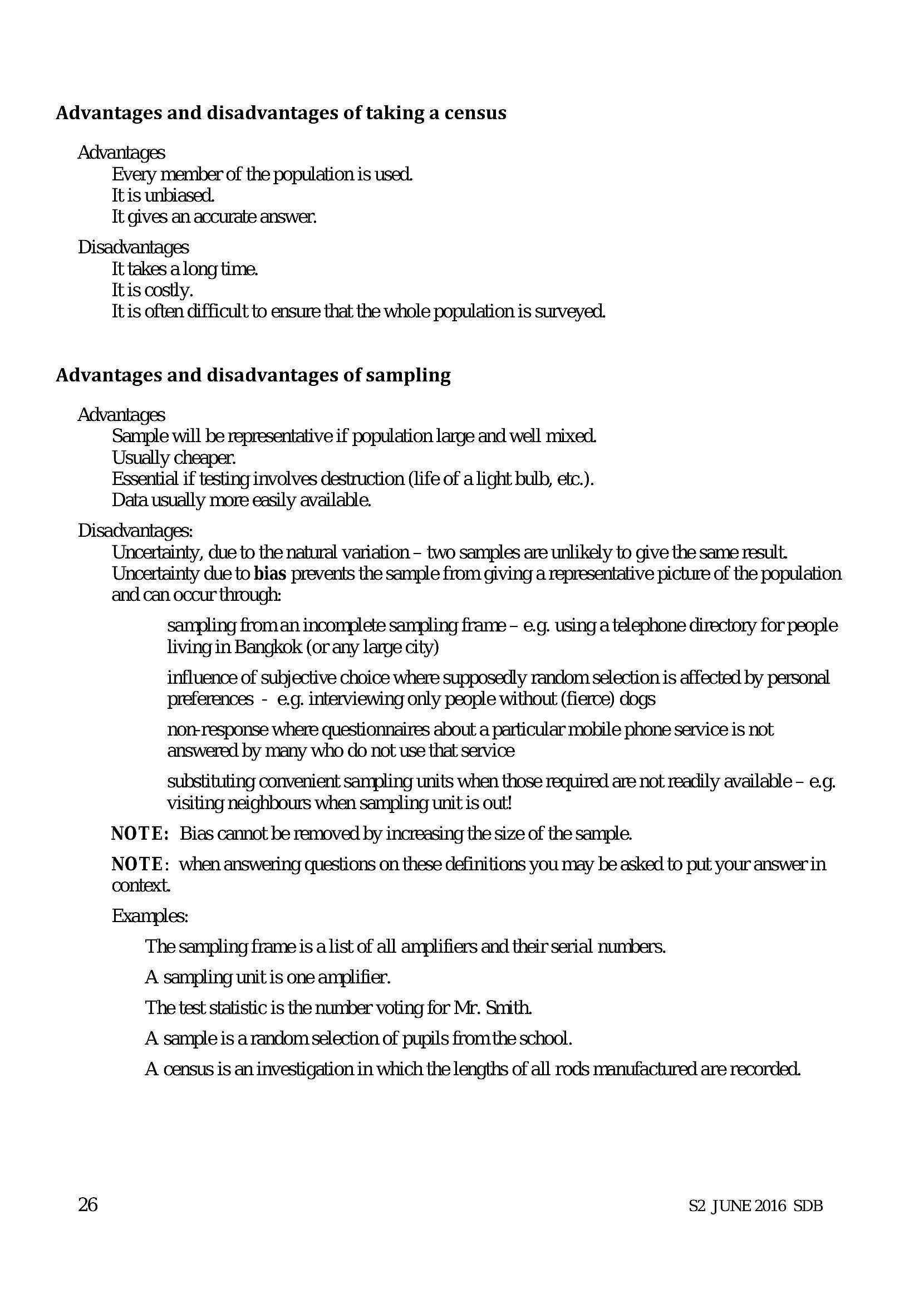
Advantages and disadvantages of taking a censusAdvantages
Every member of the population is used.
Itis unbiased.
Tt gives an accurate answer.
Disadvantages
Tt takes along time.
Itis costly.
It is often difficult to ensure that the whole population is surveyed.
Advantages and disadvantages of sampling
Advantages
Sample will be representative if population large and well mixed.
Usually cheaper.
Essential if testing involves destruction (life of a light bulb, etc.).
Data usually more easily available.
Disadvantages:
Uncertainty, due to the natural variation - two samples are unlikely to give the same result.
Uncertainty due to bias prevents the sample from giving a representative picture of the population
and can occur through:
sampling from an incomplete sampling frame - e.g. using a telephone directory for people
living in Bangkok (or any large city)
influence of subjective choice where supposedly random selection is affected by personal
preferences - eg. interviewing only people without (fierce) dogs
nor-response where questionnaires about a particular mobile phone service is not
answered by many who do not use that service
substituting convenient sampling units when those required are not readily available - e.g.
visiting neighbours when sampling unit is out!
NOTE: Bias cannot be removed by increasing the size of the sample.
NOTE: when answering questions on these definitions you may be asked to put your answer in
context.
Examples:
The sampling frame is a list of all amplifiers and their serial numbers.
A sampling unit is one amplifier.
The test statistic is the number voting for Mr. Smith.
A sample is a random selection of pupils fromthe school.
A census is an investigation in which the lengths of all rods manufactured are recorded.
26 $2 JUNE 2016 SDB
---
Page 29
Extracted Text
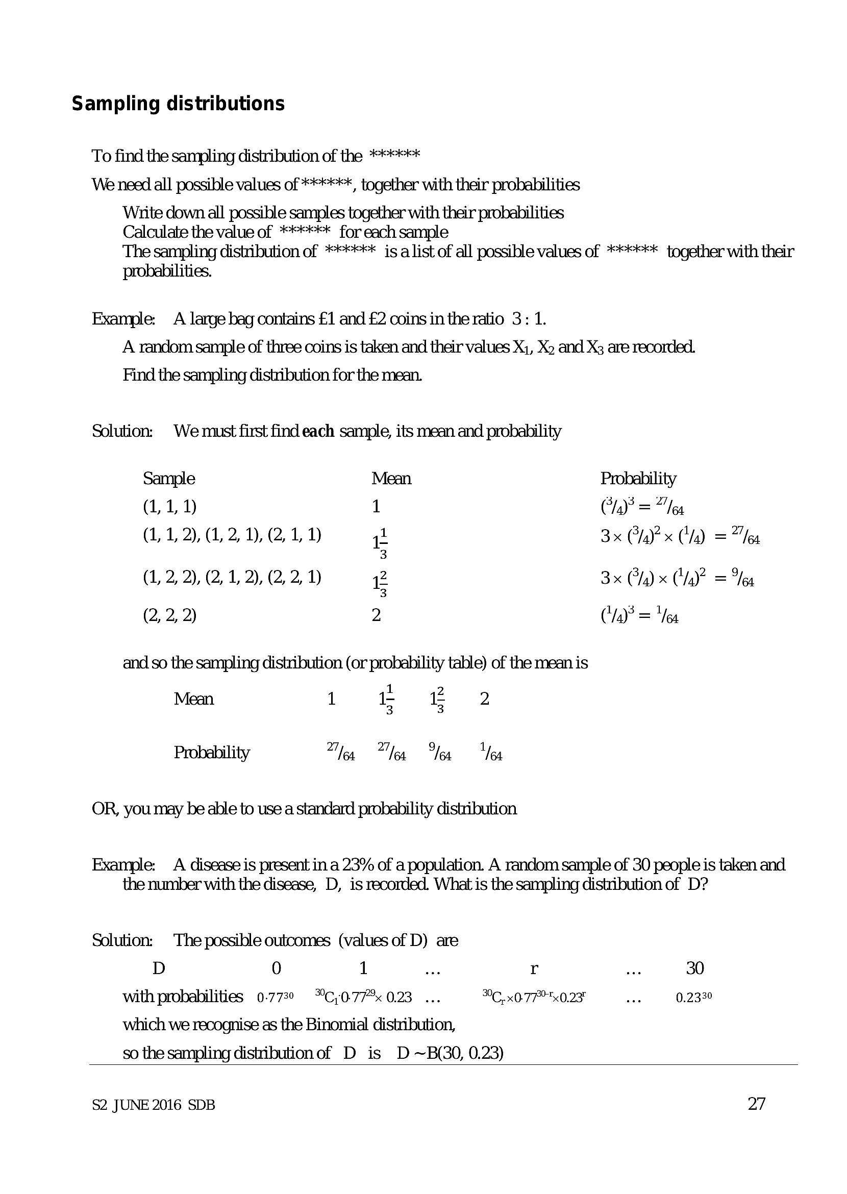
Sampling distributionsTo find the sampling distribution of the <strong></strong>**
We need all possible values of <strong></strong>**, together with their probabilities
Write down all possible samples together with their probabilities
Calculate the value of <strong></strong>** for each sample
The sampling distribution of <strong></strong><strong> is a list of all possible values of </strong><strong></strong> together with their
probahilities.
Example: A large bag contains £1 and £2 coins in the ratio 3: 1.
A random sample of three coins is taken and their values Xi, Xp and X3 are recorded.
Find the sampling distribution for the mean.
Solution: We must first find each sample, its mean and probability
Sample Mean Probability
(LL 1 Clay’ = "ea
(1, 1, 2), (1, 2, 1), (2, L 1) a 3x CPya)? x (4) = 2a
3
(1, 2, 2), (2, 1, 2), (2, 2, 1) z 3x Ca) x Cy)? = Yea
3
(2, 2, 2) 2 (“/4)? = “Yea
and so the sampling distribution (or probability table) of the mean is
Mean 1 -t £ 2
3 3
Probability ot ed (ae |
OR, you may be able to use a standard probability distribution
Example: A disease is present in a 23% of a population. A random sample of 30 people is taken and
the number with the disease, D, is recorded. What is the sampling distribution of D?
Solution: The possible outcomes (values of D) are
D 0 1 te r Le 30
with probabilities 0.7730 *C,0.77% 0.23 ... °C. x0-77° 0.23" bes 0.2330
which we recognise as the Binomial distribution,
so the sampling distributionof D is D ~B(30, 0.23)
$2 JUNE 2016 SDB 27
---
Page 30
Extracted Text
7Hypothesis tests
Null hypothesis, Ho
The hypothesis which is assumed to be correct unless shown otherwise.
Alternative hypothesis, H;
This is the conclusion that should be made if Ho is rejected
Hypothesis test
A mathematical procedure to examine a value of a population parameter proposed by the null
hypothesis, Hp compared to the altemative hypothesis, H;.
Test statistic
This is the statistic (calculated from the sample) which is tested (in cumulative probability tables,
or with the normal distribution etc.) as the last part of the significance test.
Critical region
The range of values which would lead you to reject the null hypothesis, Ho
Significance level
The actual significance level is the probability of rejecting Hp when it is in fact true.
Null and alternative hypotheses, Hy and H,
Both null and altemative hypotheses must be stated in symbols only.
The null hypothesis, Ho, is the ‘working hypothesis’, i.e. what you assume to be true for the purpose of
the test.
The altemative hypothesis, Hy, is what you conclude if you reject the null hypothesis: it also
determines whether you use a one-tail or a two-tail test.
Your conclusion must be stated in full - both in statistical language and in the context of the
question.
Hypotheses and significance level
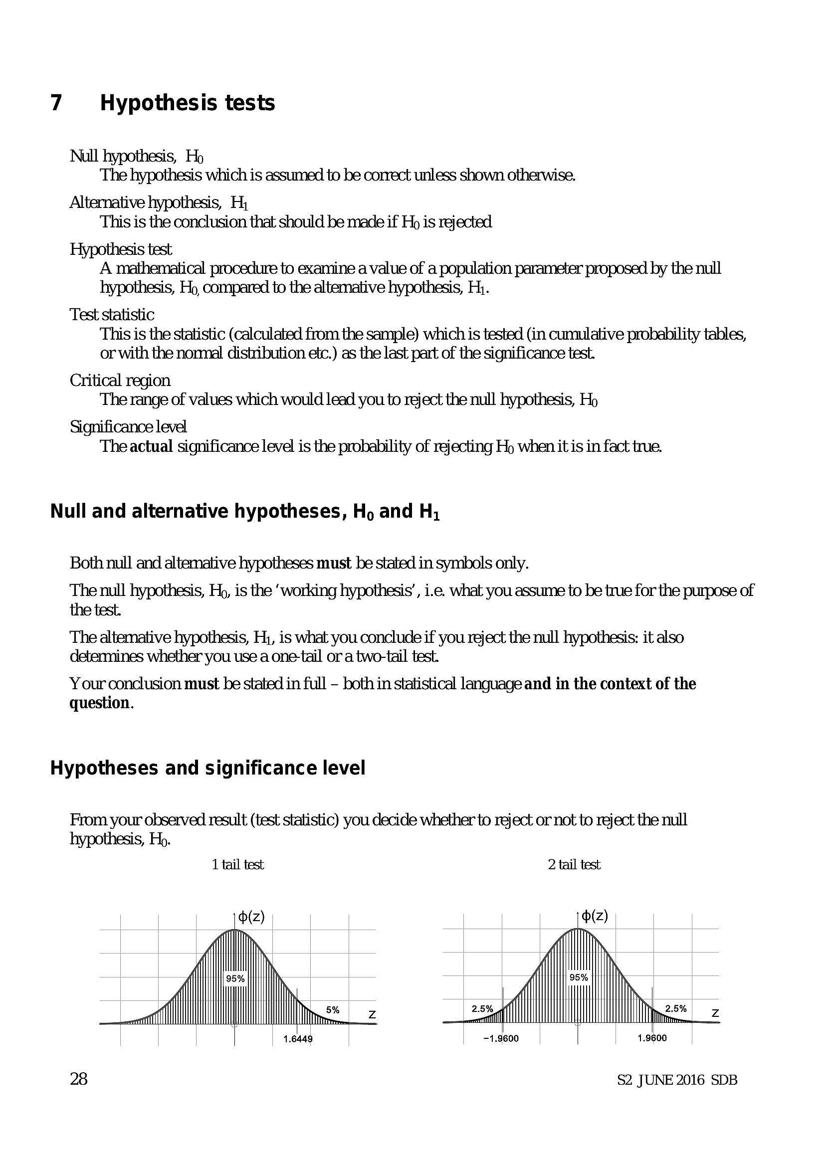
From your observed result (test statistic) you decide whether to reject or not to reject the null
hypothesis, Hp.
1 tail test 2 tail test
28 $2 JUNE 2016 SDB
---
Page 31
Extracted Text
From the null hypothesis, Ho, we could have a result anywhere on the graph - including the small (blue) shaded areas.If the observed result (test statistic) lies in a small (blue) shaded area, we say that
The test statistic is significant at 5%, or that we reject Ho. Thus Hp could actually be true but we still
reject it.
Thus, the significance level, 5%, is
the probability that we reject Hp when it is in fact true,
or the probability of incorrectly rejecting Ho.
When we reject the null hypothesis, Hp, we use the altemative hypothesis to write the conclusion.
Critical regions and significance levels
Poisson and Binomial
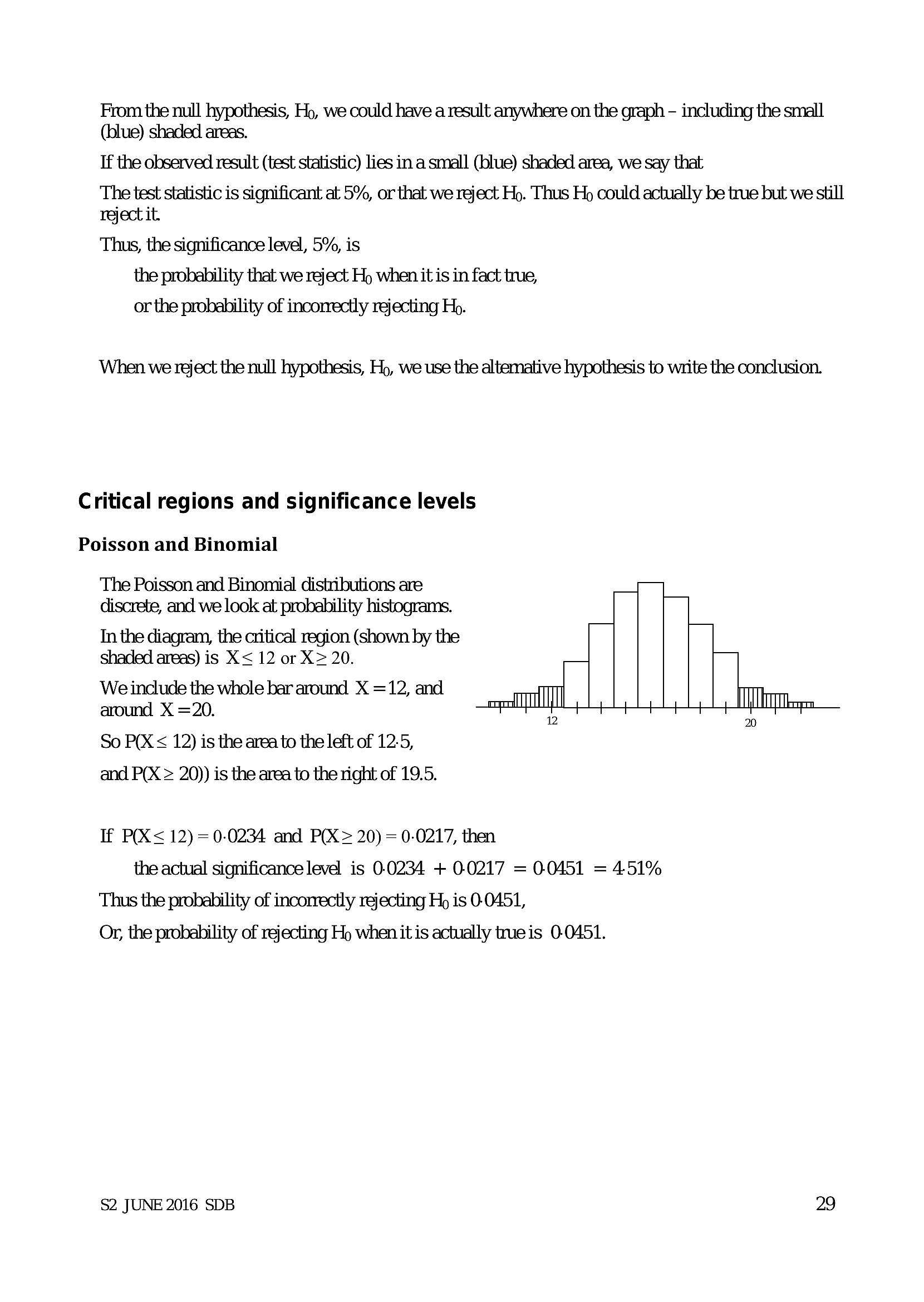
The Poisson and Binomial distributions are
discrete, and we look at probability histograms.
In the diagram, the critical region (shown by the
shaded areas) is X< 12 or X> 20.
We include the whole bar around X =12, and
around X =20.
So P(X < 12) is the area to the left of 12.5,
and P(X > 20)) is the area to the right of 19.5.
If P(X< 12) =0-0234 and P(X> 20) = 0-0217, then
the actual significance level is 0.0234 + 0.0217 = 0.0451 = 451%
Thus the probability of incomectly rejecting Hy is 0.0451,
Or, the probability of rejecting Hy when it is actually tue is 0.0451.
$2 JUNE 2016 SDB 29
---
Page 32
Extracted Text
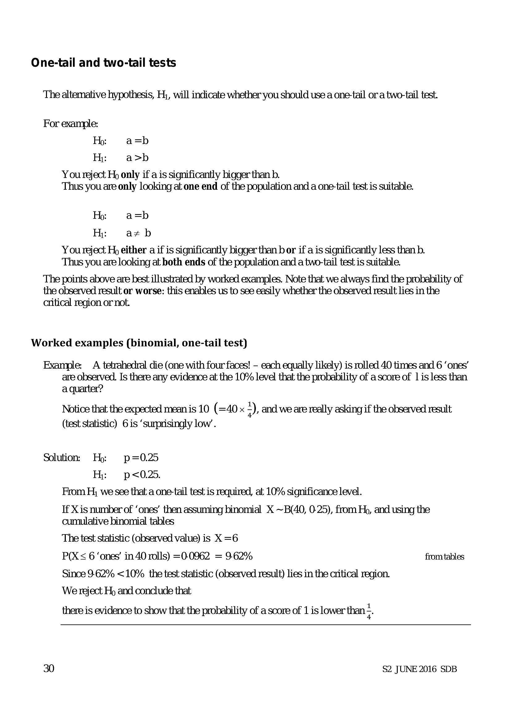
One-tail and two-tail testsThe altemative hypothesis, H;, will indicate whether you should use a one-tail or a two-tail test.
For example:
Ho: a=b
Hi: a>b
You reject Ho only if a is significantly bigger than b.
Thus you are only looking at one end of the population and a one-tail test is suitable.
Hb: a=b
Hi: a#b
You reject Hp either a if is significantly bigger than b or if a is significantly less than b.
Thus you are looking at both ends of the population and a two-tail test is suitable.
The points above are best illustrated by worked examples. Note that we always find the probability of
the observed result or worse: this enables us to see easily whether the observed result lies in the
critical region or not.
Worked examples (binomial, one-tail test)
Example: A tetrahedral die (one with four faces! - each equally likely) is rolled 40 times and 6 ‘ones’
are observed. Is there any evidence at the 10% level that the probability of a score of | is less than
a quarter?
Notice that the expected mean is 10 (=40 x *), and we are really asking if the observed result
(test statistic) 6 is ‘surprisingly low’.
Solution. Hp: p=0.25
Hi: p <0.25.
From H; we see that a one-tail test is required, at 10% significance level.
If X is number of ‘ones’ then assuming binomial X ~B(40, 0-25), from Ho, and using the
cumulative binomial tables
The test statistic (observed value) is X =6
P(X< 6 ‘ones’ in 40 rolls) =0-0962 = 9.62% from tables
Since 9.62% <10% the test statistic (observed result) lies in the critical region.
We reject Hp and conclude that
there is evidence to show that the probability of a score of 1 is lower than <.
30 $2 JUNE 2016 SDB
---
Page 33
Extracted Text
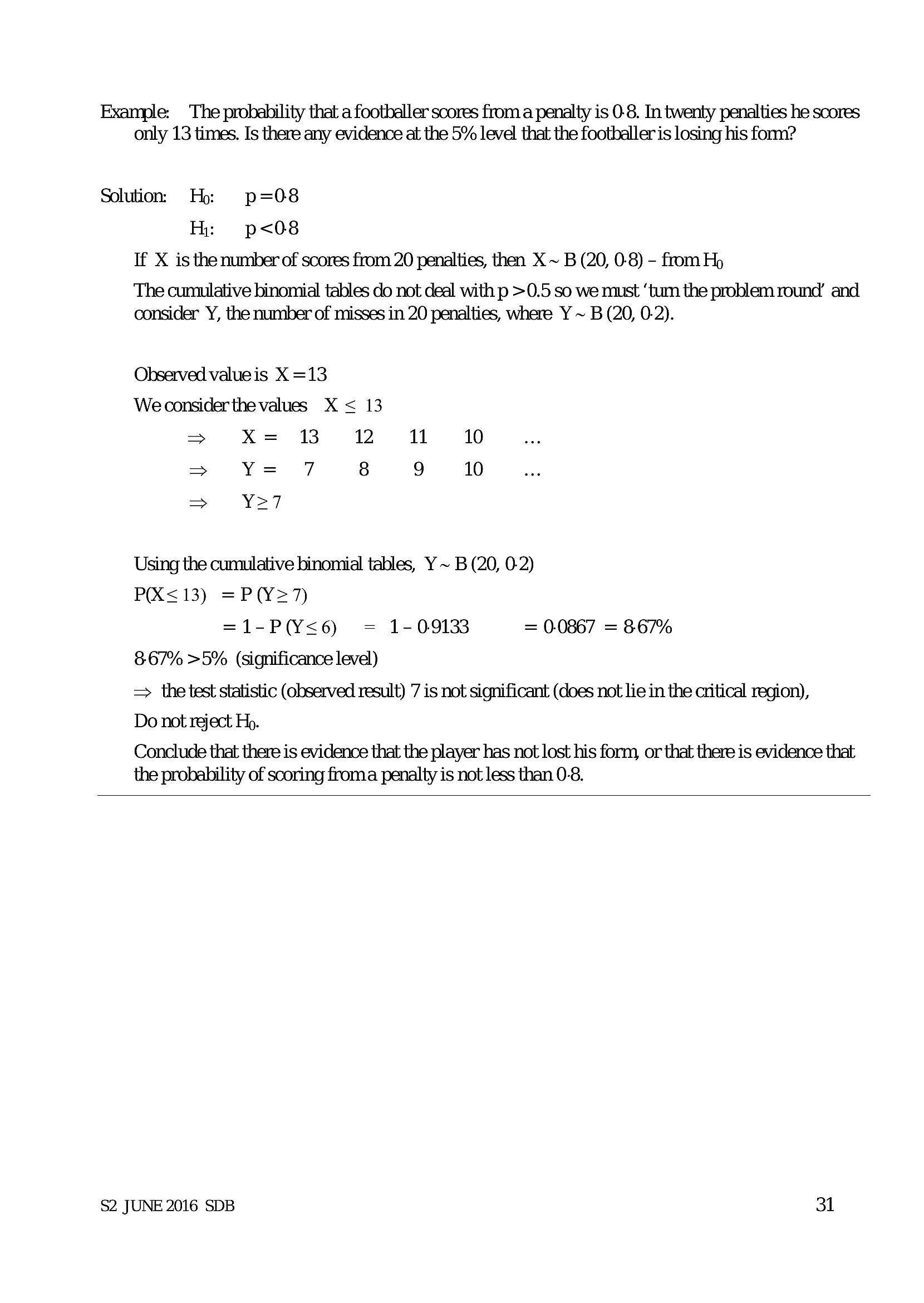
Example: The probability that a footballer scores froma penalty is 0-8. In twenty penalties he scores only 13 times. Is there any evidence at the 5% level that the footballer is losing his fon?Solution. Hp: p=08
H: p<08
If X is the number of scores from 20 penalties, then X ~ B (20, 0-8) - from Hp
The cumulative binomial tables do not deal with p >0.5 so we must ‘tum the problem round’ and
consider Y, the number of misses in 20 penalties, where Y ~ B (20, 0-2).
Observed value is X =13
We considerthe values X < 13
> X= 23 2 11 10
> Y= 7 8 9 10
=> Y>7
Using the cumulative binomial tables, Y ~ B (20, 0-2)
P(XX< 13) =P(Y>7)
=1-P(¥<6) = 1-09133 = 0.0867 = 867%
867% >5% (significance level)
=> the test statistic (observed result) 7 is not significant (does not lie in the critical region),
Do not reject Hp.
Conclude that there is evidence that the player has not lost his form, or that there is evidence that
the probability of scoring froma penalty is not less than 0-8.
$2 JUNE 2016 SDB 31
---
Page 34
Extracted Text
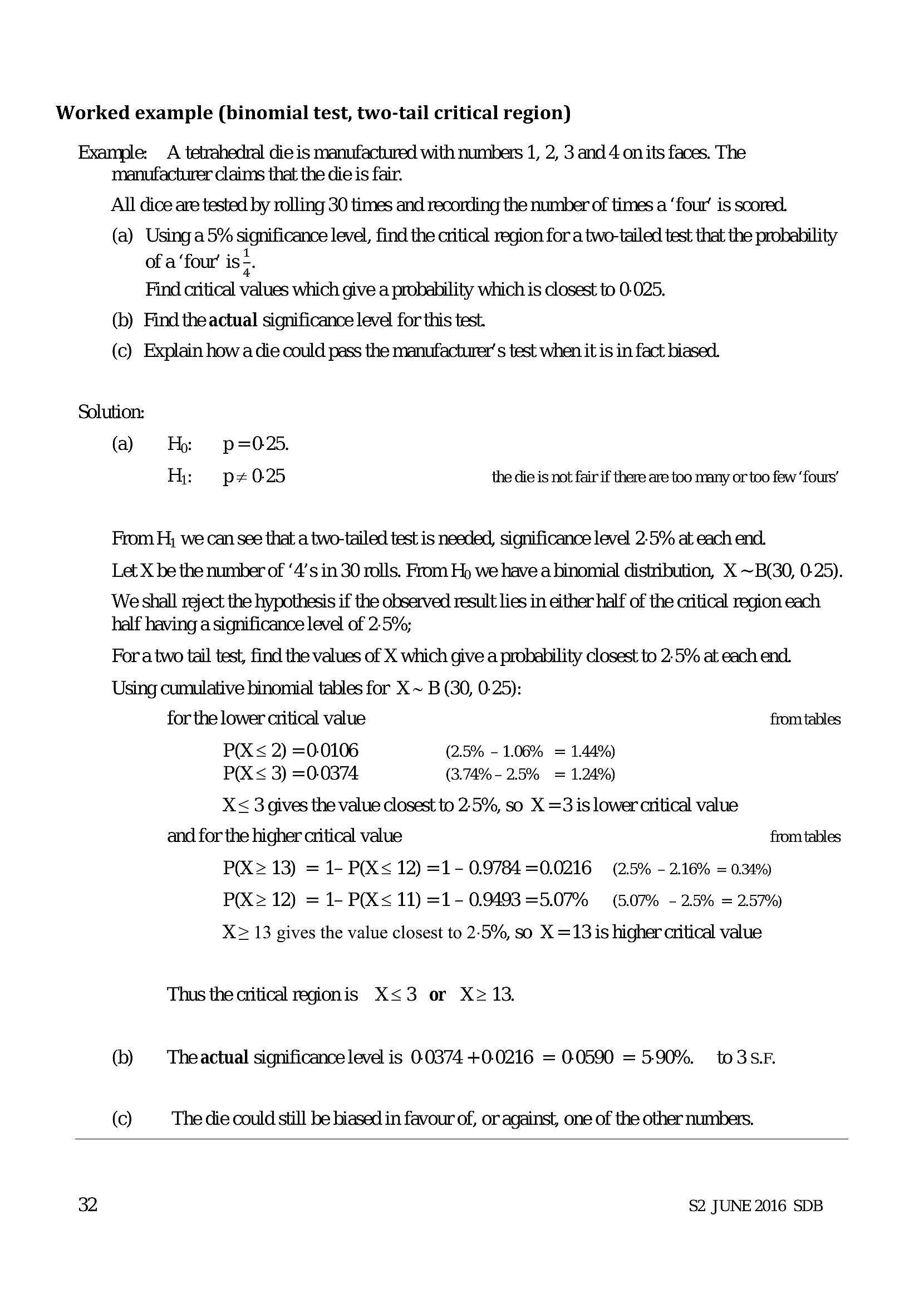
Worked example (binomial test, two-tail critical region) Example: A tetrahedral die is manufactured with numbers 1, 2, 3 and 4 on its faces. Themanufacturer claims that the die is fair.
All dice are tested by rolling 30 times and recording the number of times a ‘four’ is scored.
(a) Using a5% significance level, find the critical region for a two-tailed test that the probability
of a ‘four’ is =.
Find critical values which give a probability which is closest to 0-025.
(b) Find the actual significance level for this test.
(c) Explain how a die could pass the manufacturer’ s test when it is in fact biased.
Solution:
(a) Hp: p=025.
Hy: p#025 the die is not fair if there are too many or too few ‘fours’
From H, we can see that a two-tailed test is needed, significance level 2.5% at each end.
Let X be the number of ‘4’s in 30 rolls. From Hp we have a binomial distribution, X ~B(30, 0-25).
We shall reject the hypothesis if the observed result lies in either half of the critical region each
half having a significance level of 2:5%;
Fora two tail test, find the values of X which give a probability closest to 2.5% at each end.
Using cumulative binomial tables for X ~ B (30, 0-25):
for the lower critical value from tables
P(X < 2) =0-0106 (2.5% - 1.06% = 1.44%)
P(X < 3) =0.0374 (3.74% - 2.5% = 1.24%)
X< 3 gives the value closest to 2.5%, so X =3 is lower critical value
and for the higher critical value from tables
P(X= 13) = 1- P(XX< 12) =1- 0.9784 =0.0216 (2.5% - 2.16% = 0.4%)
P(X> 12) = 1- P(X¥< 11) =1- 0.9493 =5.07% (5.07% - 2.5% = 2.57%)
X> 13 gives the value closest to 2:5%, so X =13 is higher critical value
Thus the cntical regionis X<3 or X> 13.
(b) Theactual significance level is 0.0374 +0-0216 = 0.0590 =590%. to3s.F
(c) The die could still be biased in favour of, or against, one of the other numbers.
32 $2 JUNE 2016 SDB
---
Page 35
Extracted Text
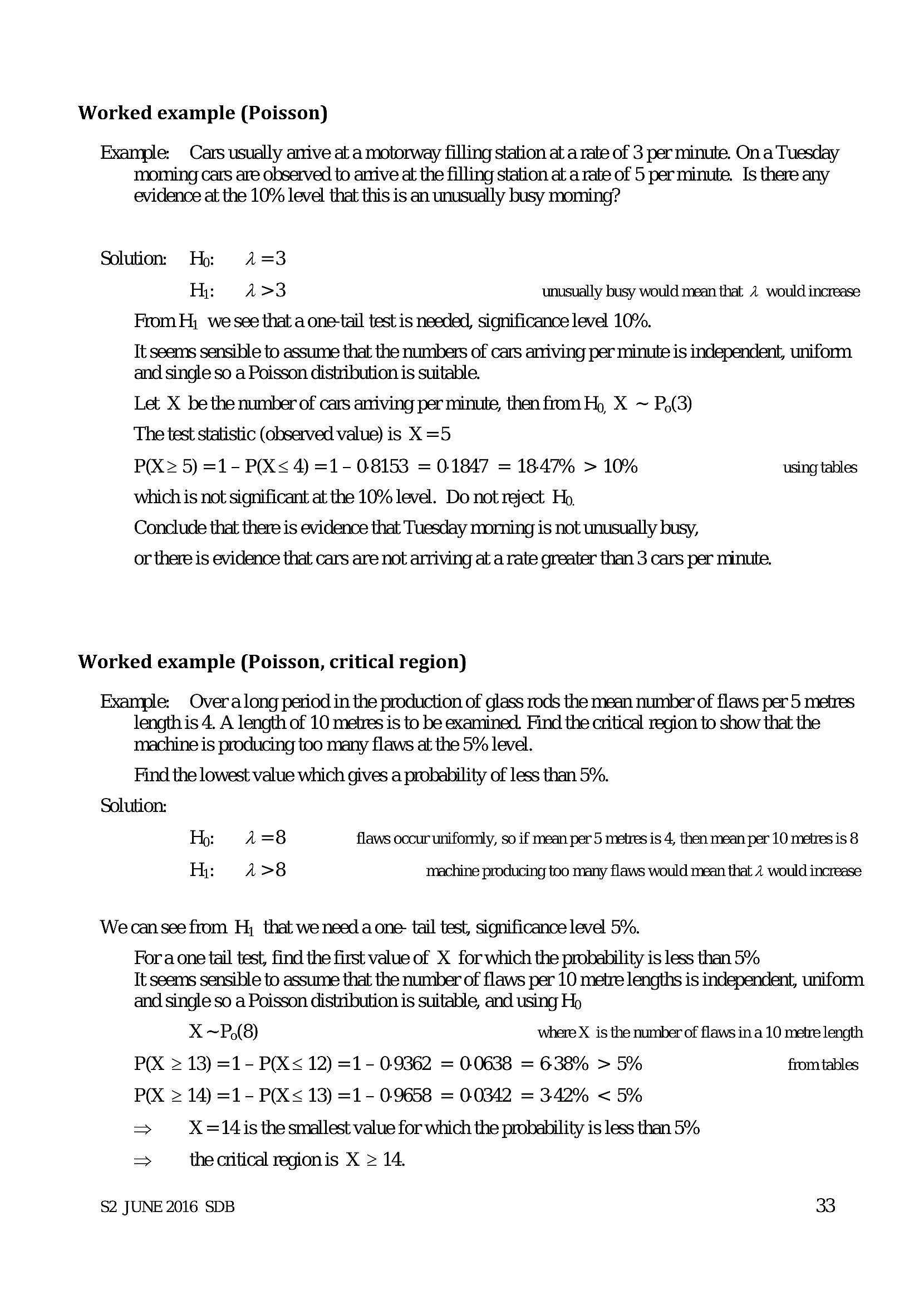
Worked example (Poisson)Example: Cars usually arrive at a motorway filling station at a rate of 3 per minute. On a Tuesday
moming cars are observed to anive at the filling station at a rate of 5 perminute. Is there any
evidence at the 10% level that this is an unusually busy moming?
Solution. Hj: 4=3
H: Aa>3 unusually busy would mean that 2 would increase
From H; we see that a one-tail test is needed, significance level 10%.
Tt seems sensible to assume that the numbers of cars arriving per minute is independent, uniform
and single so a Poisson distribution is suitable.
Let X be the number of cars arriving per minute, then from Hp X ~ P,(3)
The test statistic (observed value) is X =5
P(X 5) =1- P(X< 4) =1- 08153 = 01847 = 18.47% > 10% using tables
which is not significant at the 10% level. Do not reject Ho.
Conclude that there is evidence that Tuesday morning is not unusually busy,
or there is evidence that cars are not arriving at a rate greater than 3 cars per minute.
Worked example (Poisson, critical region)
Example: Overalong period in the production of glass rods the mean number of flaws per 5 metres
length is 4. A length of 10 metres is to be examined. Find the critical region to show that the
machine is producing too many flaws at the 5% level.
Find the lowest value which gives a probability of less than 5%.
Solution:
H: Aa=8 flaws occur unifonmly, so if mean per 5 metres is 4, then mean per 10 metres is 8
H: Aa>8 machine producing too many flaws would mean that 2 would increase
We can see from H, that we need a one- tail test, significance level 5%.
Fora one tail test, find the first value of X for which the probability is less than 5%
Tt seems sensible to assume that the number of flaws per 10 metre lengths is independent, uniform
and single so a Poisson distribution is suitable, and using Ho
X ~P,(8) where X is the number of flaws in a 10 metre length
P(X = 13) =1- PX< 12) =1- 09362 = 0.0638 = 638% > 5% from tables
P(X = 14) =1- P< 13) =1- 09658 = 0.0342 = 342% < 5%
> X =14 is the smallest value for which the probability is less than 5%
> the critical regionis X > 14.
$2 JUNE 2016 SDB 33
---
Page 36
Extracted Text
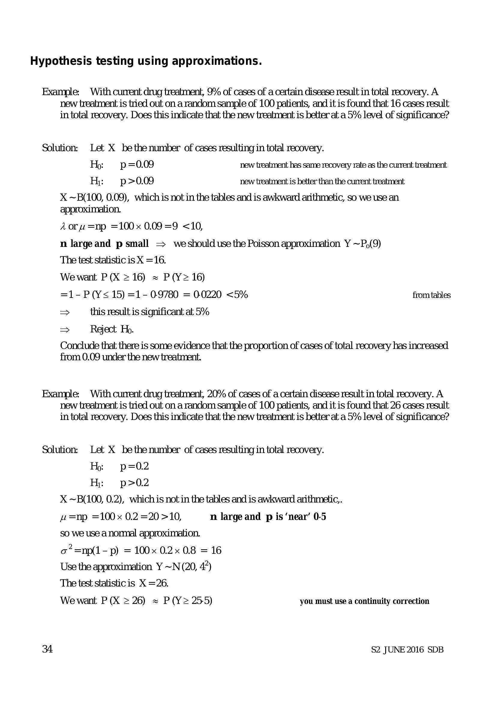
Hypothesis testing using approximations.Example: With current drug treatment, 9% of cases of a certain disease result in total recovery. A
new treatment is tried out on a random sample of 100 patients, and it is found that 16 cases result
in total recovery. Does this indicate that the new treatment is better at a 5% level of significance?
Solution: Let X bethe number of cases resulting in total recovery.
Hp: p=0.09 new treatment has same recovery rate as the current treatment
H;: p>0.09 new treatment is better than the current treatment
X ~B(100, 0.09), which is not in the tables and is awkward arithmetic, so we use an
approximation.
Aoru =np =100~x 0.09 =9 <10,
n large and p small = weshould use the Poisson approximation Y ~P,(9)
The test statistic is X =16.
Wewant P(X > 16) =~ P(Y> 16)
=1-P(¥< 15) =1- 09780 = 00220 <5% from tables
> this result is significant at 5%
Conclude that there is some evidence that the proportion of cases of total recovery has increased.
from 0.09 under the new treatment.
Example: With current drug treatment, 20% of cases of a certain disease result in total recovery. A
new treatment is tried out on a random sample of 100 patients, and it is found that 26 cases result
in total recovery. Does this indicate that the new treatment is better at a 5% level of significance?
Solution: Let X bethe number of cases resulting in total recovery.
H: p=0.2
H: p>02
X ~B(100, 0.2), which is not in the tables and is awkward arithmetic,.
#=np =100~x 0.2 =20 >10, n large and p is ‘near’ 0-5
so we use a nonnal approximation.
o =np(1- p) = 100x 0.2 0.8 = 16
Use the approximation Y ~N (20, 4?)
The test statistic is X =26.
We want P (X > 26) ~ P(Y> 25-5) you must use a continuity correction
34 $2 JUNE 2016 SDB
---
Page 37
Extracted Text
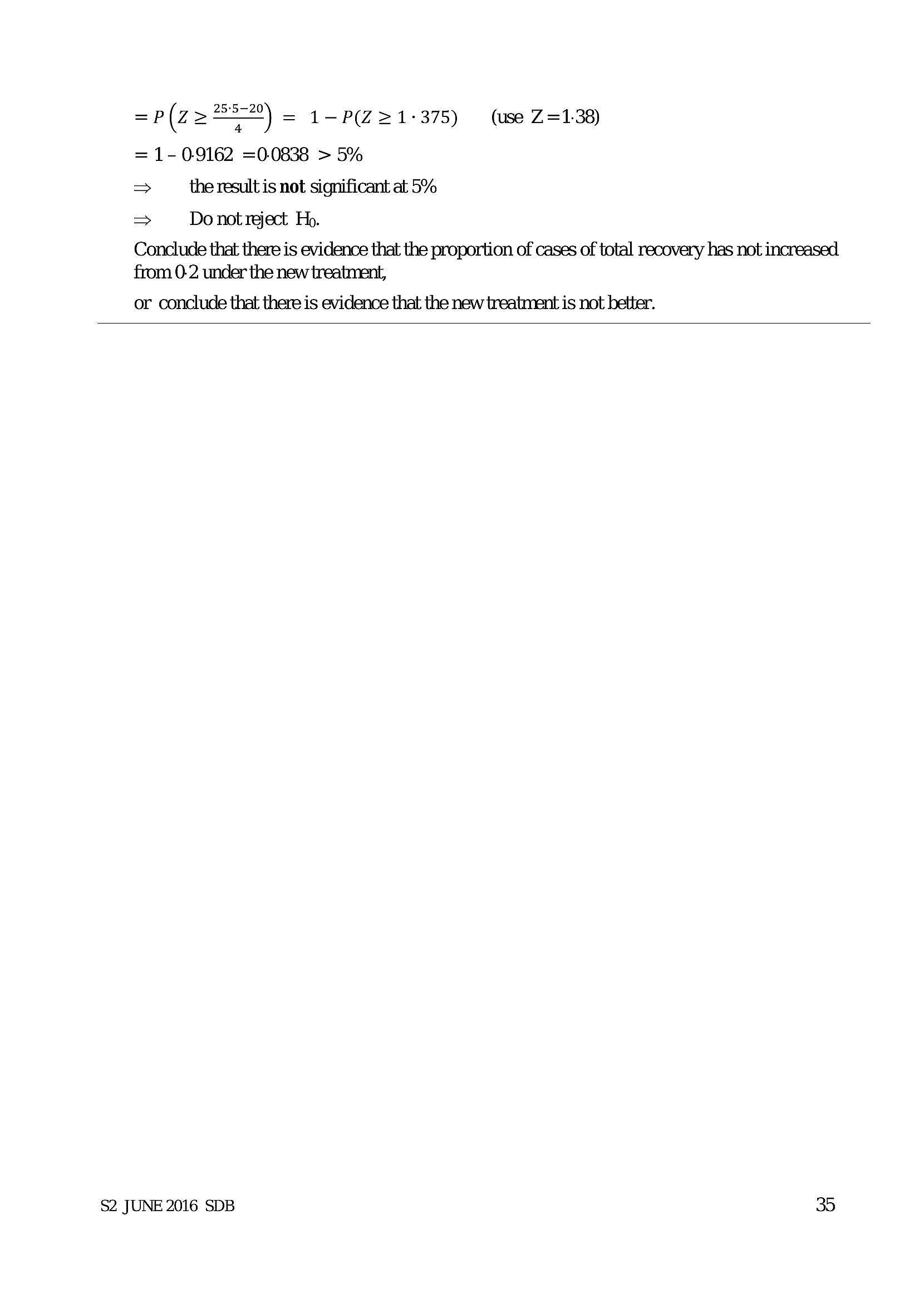
=P(z> 7°) = 1-PZ 21-375) (use Z=1.38) = 1-0-9162 =0.0838 > 5% > the result is not significant at 5%> Do not reject Ho.
Conclude that there is evidence that the proportion of cases of total recovery has not increased
from 0-2 under the new treatment,
or conclude that there is evidence that the new treatment is not better.
$2 JUNE 2016 SDB 35
---
Page 38
Extracted Text
8 Context questions and answersAccuracy
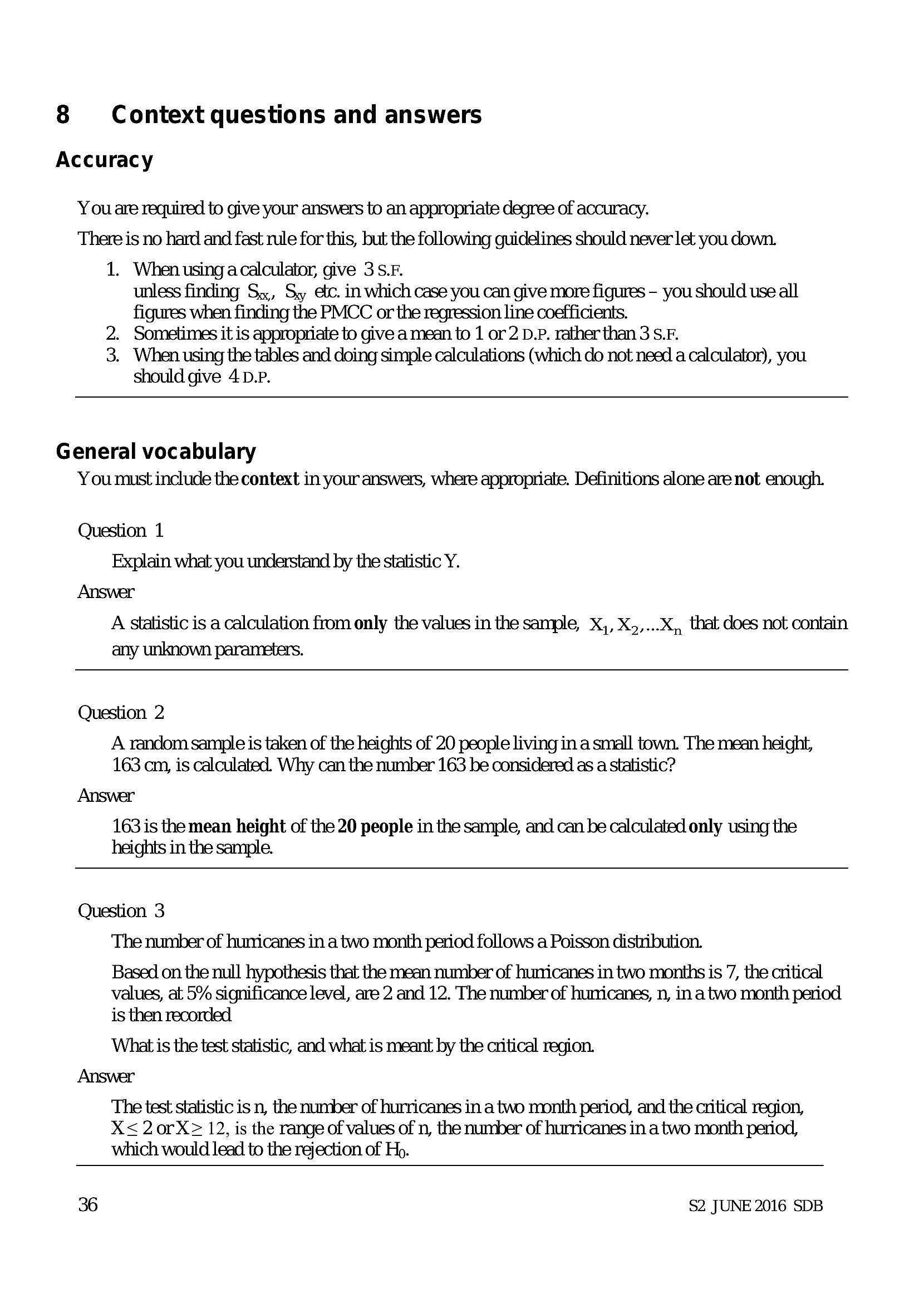
You are required to give your answers to an appropriate degree of accuracy.
There is no hard and fast rule for this, but the following guidelines should never let you down.
1. When using a calculator, give 3 S.F.
unless finding Sx, Sy etc. in which case you can give more figures — you should use all
figures when finding the PMCC or the regression line coefficients.
2. Sometimes it is appropnate to give a mean to 1 or 2 D.P. rather than 3 S.F.
3. When using the tables and doing simple calculations (which do not need a calculator), you
should give 4 D.P.
General vocabulary
You must include the context in your answers, where appropriate. Definitions alone are not enough.
Question 1
Explain what you understand by the statistic Y.
Answer
A statistic is a calculation from only the values in the sample, X,, X,,...X,, that does not contain
any unknown parameters.
Question 2
A random sample is taken of the heights of 20 people living in a small town. The mean height,
163 cm, is calculated. Why can the number 163 be considered as a statistic?
Answer
163 is the mean height of the 20 people in the sample, and can be calculated only using the
heights in the sample.
Question 3
The number of hurricanes in a two month period follows a Poisson distribution.
Based on the null hypothesis that the mean number of hurricanes in two months is 7, the critical
values, at 5% significance level, are 2 and 12. The number of hunricanes, n, in a two month period
is then recorded
What is the test statistic, and what is meant by the critical region.
Answer
The test statistic is n, the number of hurricanes in a two month period, and the critical region,
X< 2orX> 12, is the range of values of n, the number of hurricanes in a two month period,
which would lead to the rejection of Hp.
36 $2 JUNE 2016 SDB
---
Page 39
Extracted Text
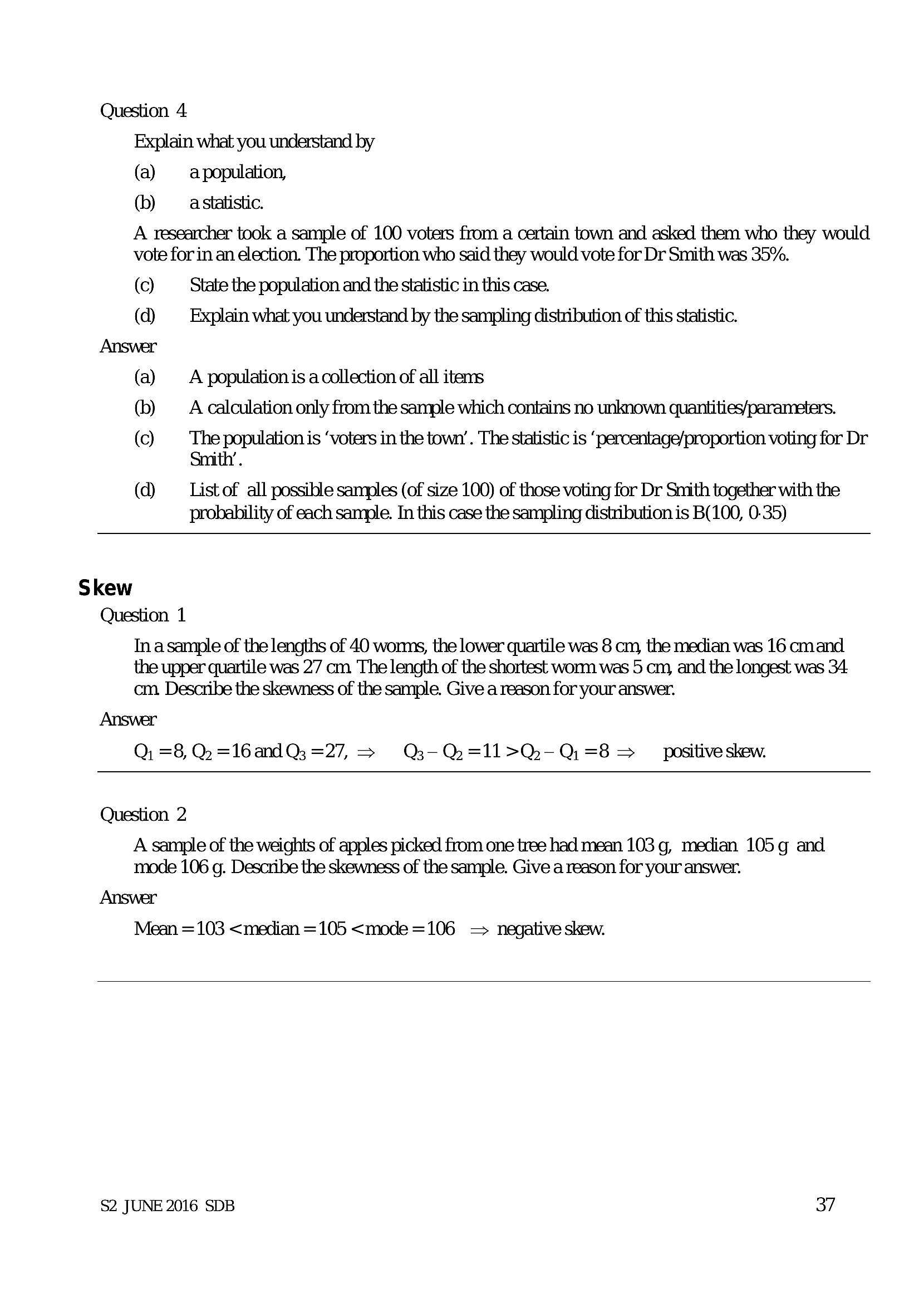
Question 4Explain what you understand by
(a) a population,
(b) a statistic.
A researcher took a sample of 100 voters from a certain town and asked them who they would
vote for in an election. The proportion who said they would vote for Dr Smith was 35%.
(c) State the population and the statistic in this case.
(d) — Explain what you understand by the sampling distribution of this statistic.
Answer
(a) A population is a collection of all items
(b) =A calculation only from the sample which contains no unknown quantities/parameters.
(c) we population is ‘voters in the town’ . The statistic is ‘percentage/proportion voting for Dr
(d) List of all possible samples (of size 100) of those voting for Dr Smith together with the
probability of each sample. In this case the sampling distribution is B(100, 0-35)
Skew
Question 1
In asample of the lengths of 40 womms, the lower quartile was 8 cm, the median was 16 cmand
the upper quartile was 27 cm The length of the shortest wonn was 5 cm, and the longest was 34
cm. Describe the skewness of the sample. Give a reason for your answer.
Answer
Q, =8, Q =16 andQ3 =27, > Q-Q=11>Q-Q=8 positive skew.
Question 2
A sample of the weights of apples picked from one tree had mean 103 g, median 105g and
mode 106 g. Describe the skewness of the sample. Give a reason for your answer.
Answer
Mean = 103 <median =105 <mode=106 = negative skew.
$2 JUNE 2016 SDB 37
---
Page 40
Extracted Text
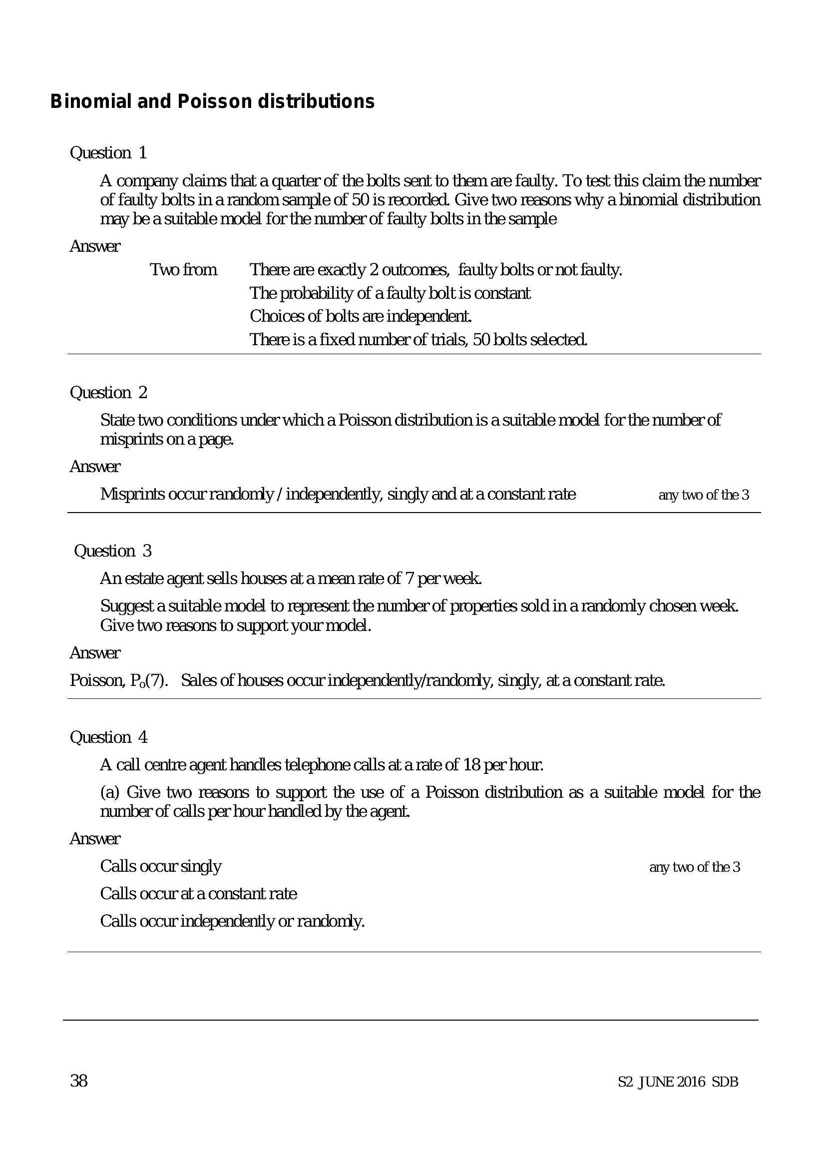
Binomial and Poisson distributionsQuestion 1
A company claims that a quarter of the bolts sent to them are faulty. To test this claim the number
of faulty bolts in a random sample of 50 is recorded. Give two reasons why a binomial distribution
may be a suitable model for the number of faulty bolts in the sample
Answer
Twofrom ‘There are exactly 2 outcomes, faulty bolts or not faulty.
The probability of a faulty bolt is constant
Choices of bolts are independent.
There is a fixed number of trials, 50 bolts selected.
Question 2
State two conditions under which a Poisson distribution is a suitable model for the number of
misprints on a page.
Answer
Misprints occurrandomly / independently, singly and at a constant rate any two of the 3
Question 3
An estate agent sells houses at a mean rate of 7 per week.
Suggest a suitable model to represent the number of properties sold in a randomly chosen week.
Give two reasons to support your model.
Answer
Poisson, P,(7). Sales of houses occur independently/randomly, singly, at a constant rate.
Question 4
A call centre agent handles telephone calls at a rate of 18 per hour.
(a) Give two reasons to support the use of a Poisson distribution as a suitable model for the
number of calls per hour handled by the agent.
Answer
Calls occur singly any two of the 3
Calls occur at a constant rate
Calls occur independently or randomly.
38 $2 JUNE 2016 SDB
---
Page 41
Extracted Text
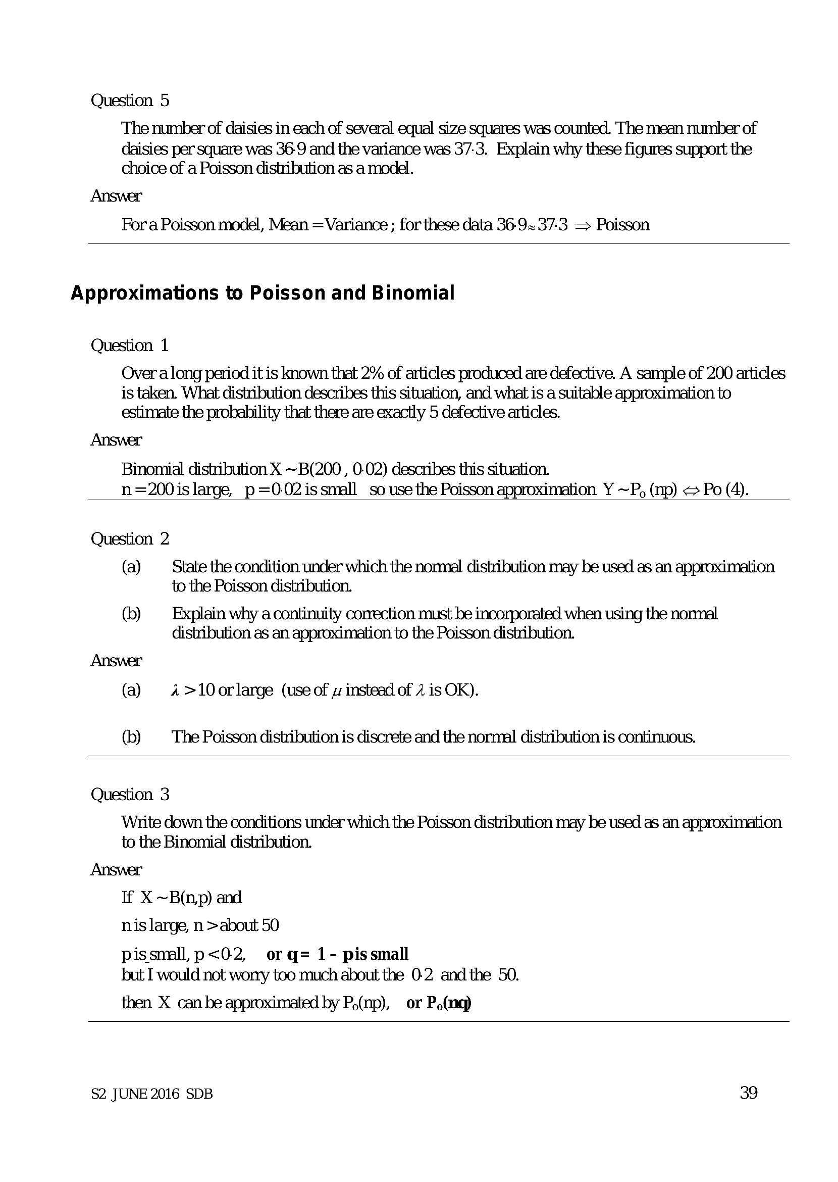
Question 5The number of daisies in each of several equal size squares was counted. The mean number of
daisies per square was 36.9 and the variance was 37-3. Explain why these figures support the
choice of a Poisson distribution as a model.
Answer
Fora Poisson model, Mean = Variance ; for these data 36-9~ 37:3 — Poisson
Approximations to Poisson and Binomial
Question 1
Over along pexiod it is known that 2% of articles produced are defective. A sample of 200 articles
is taken. What distribution describes this situation, and what is a suitable approximation to
estimate the probability that there are exactly 5 defective articles.
Answer
Binomial distribution X ~B(200 , 0-02) describes this situation.
n=200is large, p=0-02issmall so use the Poisson approximation Y ~P, (np) < Po (4).
Question 2
(a) State the condition under which the normal distribution may be used as an approximation
to the Poisson distribution.
(b) Explain why acontinuity correction must be incorporated when using the normal
distribution as an approximation to the Poisson distribution.
Answer
(a) Aa>10orlarge (use of . instead of 2 is OK).
(b) The Poisson distribution is discrete and the normal distribution is continuous.
Question 3
Write down the conditions under which the Poisson distribution may be used as an approximation
to the Binomial distribution.
Answer
If X ~B(n,p) and
nis large, n >about 50
pissmall, p<0-2, or q= 1- pissmall
but I would not worry too much about the 0-2 and the 50.
then X can be approximated by P,(np), or P»(nq)
$2 JUNE 2016 SDB 39
---
Page 42
Extracted Text
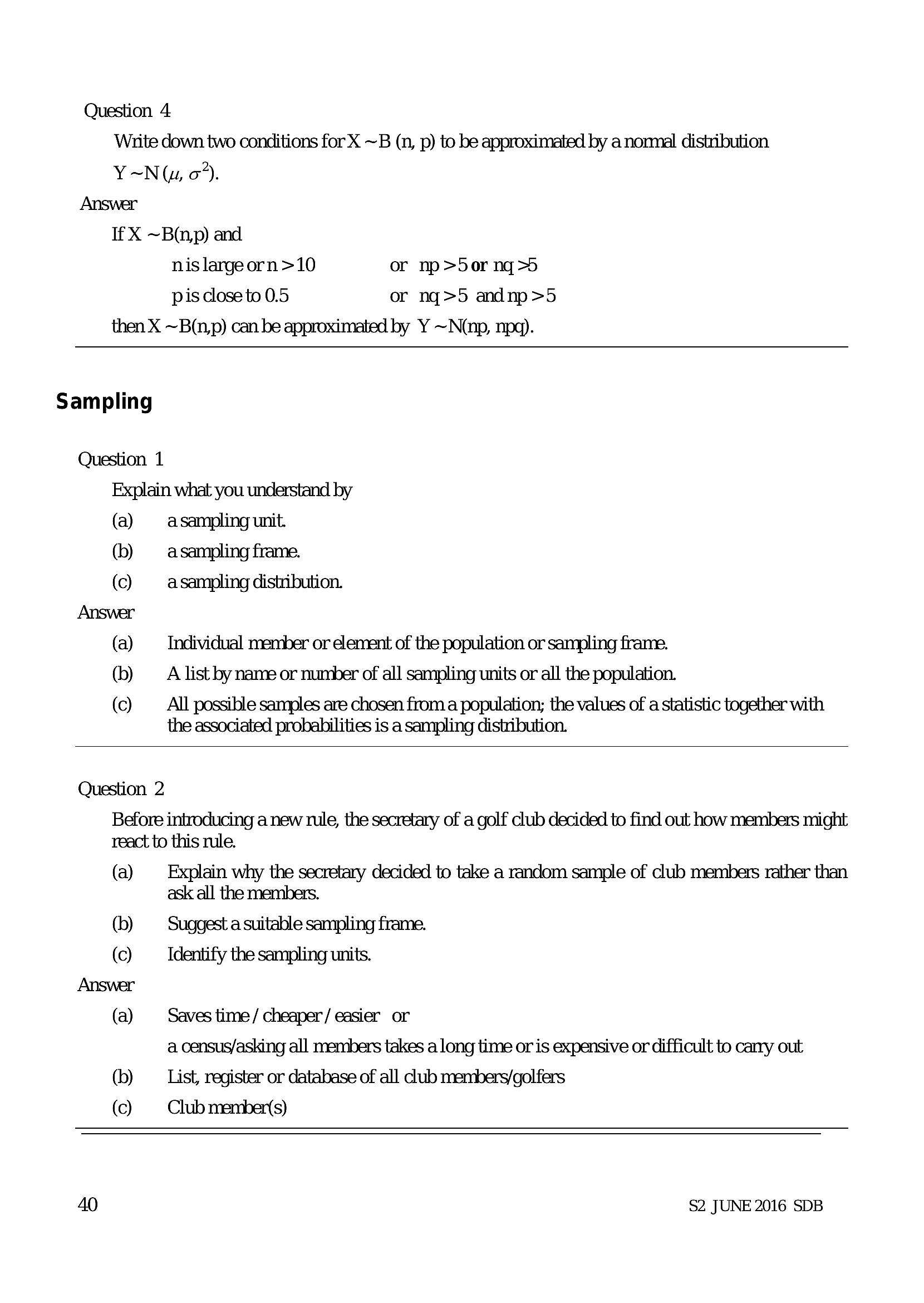
Question 4 Write down two conditions for X ~B (n, p) to be approximated by a nommal distributionY~N(u, o°).
Answer
If X ~B(n,p) and
nis largeorn>10 or np>5or nqg>5
pis close to 0.5 or nq>5 andnp>5
then X ~B(n,p) can be approximated by Y ~N(np, npq).
Sampling
Question 1
Explain what you understand by
(a) asampling unit.
(b) asampling frame.
(c) asampling distribution.
Answer
(a) —_ Individual member or element of the population or sampling frame.
(b) —_ A list by name or number of all sampling units or all the population.
(c) _ All possible samples are chosen froma population; the values of a statistic together with
the associated probabilities is a sampling distribution.
Question 2
Before introducing a new tule, the secretary of a golf club decided to find out how members might
react to this rule.
(a) Explain why the secretary decided to take a random sample of club members rather than
ask all the members.
(b) Suggest a suitable sampling frame.
(c) Identify the sampling units.
(a) Saves time/ cheaper/ easier or
a census/asking all members takes a long time or is expensive or difficult to carry out
(b) List, register or database of all club members/golfers
(c) Club member(s)
40 $2 JUNE 2016 SDB
---
Page 43
Extracted Text
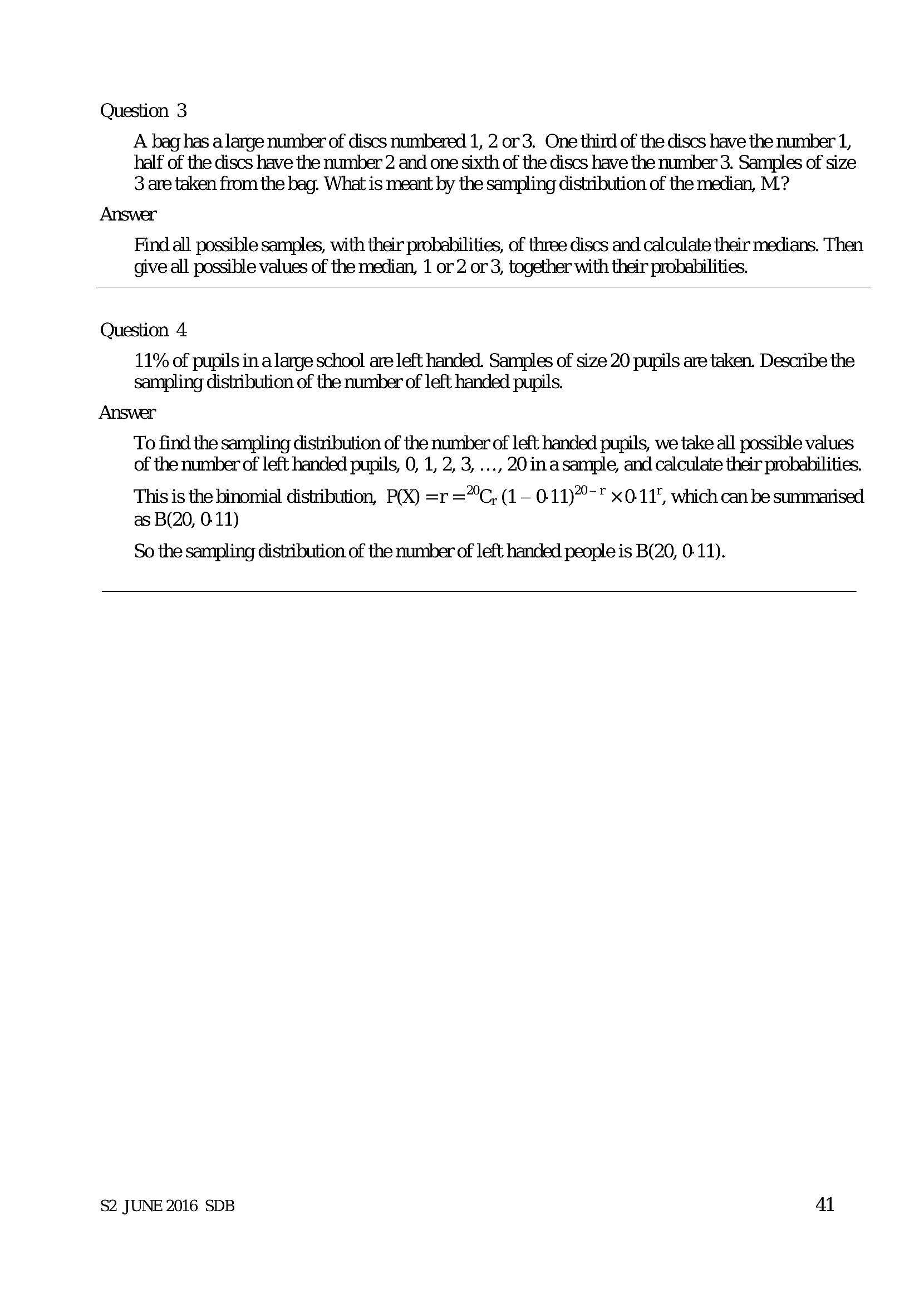
Question 3A bag has a large number of discs numbered 1, 2 or 3. One third of the discs have the number 1,
half of the discs have the number 2 and one sixth of the discs have the number 3. Samples of size
3 are taken from the bag. What is meant by the sampling distribution of the median, M.?
Answer
Find all possible samples, with their probabilities, of three discs and calculate their medians. Then
give all possible values of the median, 1 or 2 or 3, together with their probabilities.
Question 4
11% of pupils in a large school are left handed. Samples of size 20 pupils are taken. Describe the
sampling distribution of the number of left handed pupils.
Answer
To find the sampling distribution of the number of left handed pupils, we take all possible values
of the number of left handed pupils, 0, 1, 2, 3, ..., 20 in asample, and calculate their probabilities.
This is the binomial distribution, P(X) =r ="°C, (1— 0-11)°-* x0-11', which can be summarised
as B(20, 0-11)
So the sampling distribution of the number of left handed people is B(20, 0-11).
$2 JUNE 2016 SDB Al
---
Page 44
Extracted Text
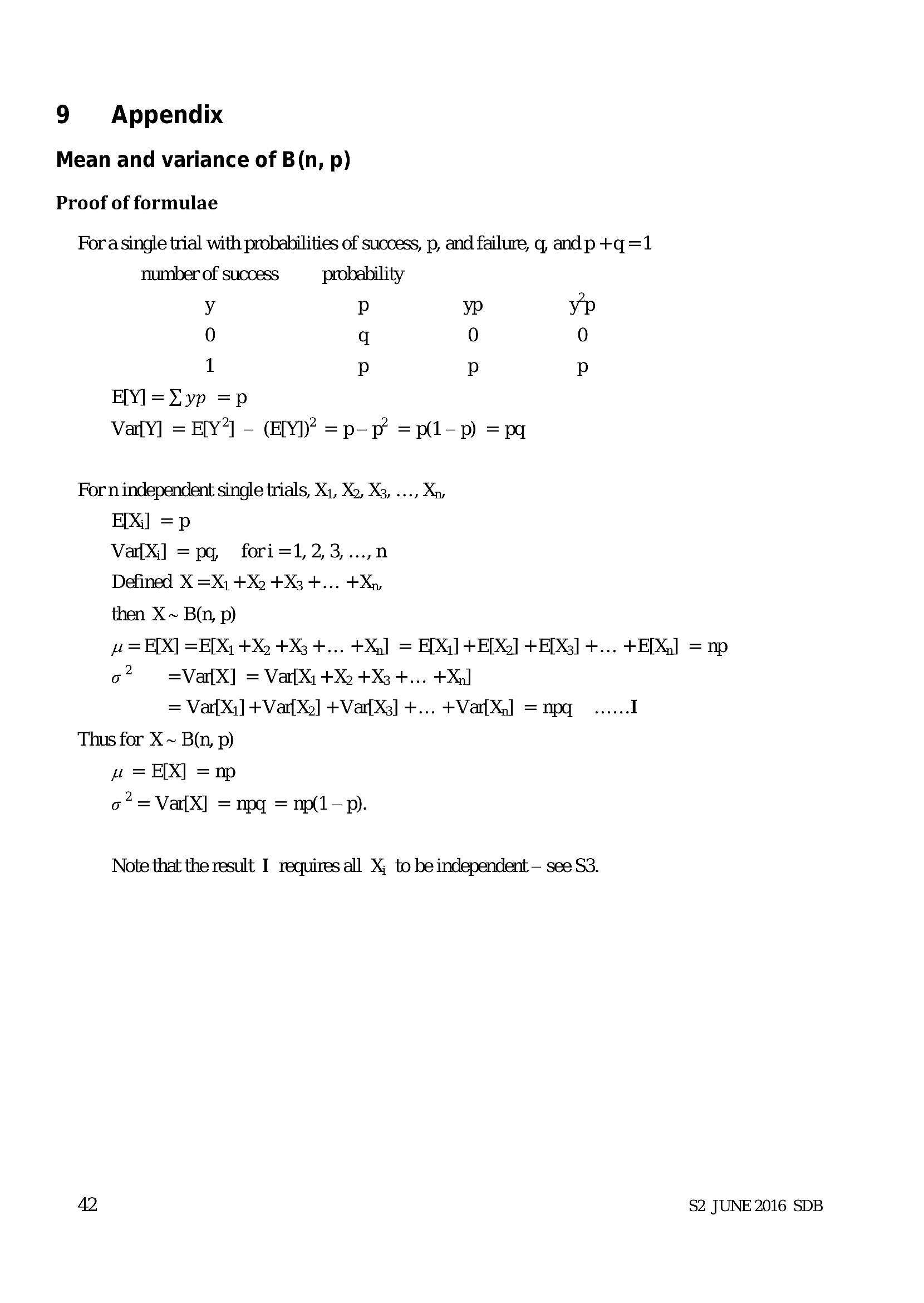
9 Appendix Mean and variance of B(n, p)Proof of formulae
Fora single trial with probabilities of success, p, and failure, q, andp +q=1
number of success probability
y p yp yp
0 q 0 0
1 Pp Pp p
HY] =X yp =p
VatY] = E[Y’] - (EIY)? =p-p =p-p) =pq
For n independent single trials, Xi, Xo, X3, ..., Xn,
HX] =p
VatX] =pq, fori=1,2,3,...,.n
Defined X =X; +X2 +X3 +... +Xn,
then X ~ Bin, p)
i = E[X] =E[X, +X) +X3 +... +X] = E[X)] + ED] +E[X3] +... + EDG]
o? =VafX] = VartXi +X2 +X3 +... +Xal
= Var Xi] + Var Xo] +VarX3] +... +VarX:] =npq ...... I
Thus for X ~ Bn, p)
<h3 class="text-primary mt-4 mb-2">= EX] =np</h3>
o?=Va{X] = npg = np(1-p).
Note that the result I requires all X; to be independent — see S3.
= np
$2 JUNE 2016 SDB
---
Page 45
Extracted Text
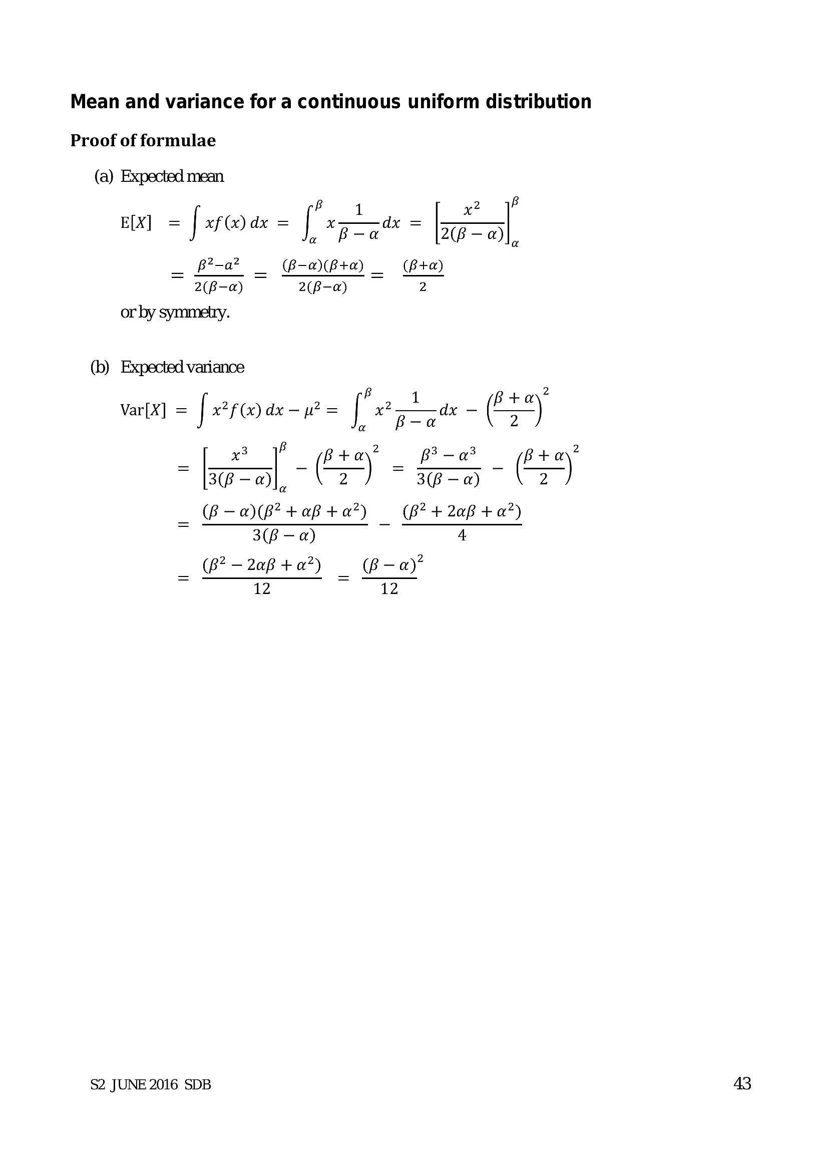
Mean and variance for a continuous uniform distribution Proof of formulae(a) Expected mean
B 1 2 B
E[X] = [ 7@ a = | Rag = Laal
B-a _ (B-a)(B+a) _ (B+a)
2(B-a) a B-a) 2
or by symmetry.
(b) Expected variance
B 2
Var[X] = [ er@ar- = [ Pond - (*)
3 B 2 3 2
- Gal -O - SS - OS
(B-a)(P?tab+a<em>) (Br +2afp +a</em>)
3(B — a) 4
_ (6? -2aB +07) — (B-a)’
~ 12 ~ 12
$2 JUNE 2016 SDB
---
Page 46
Extracted Text
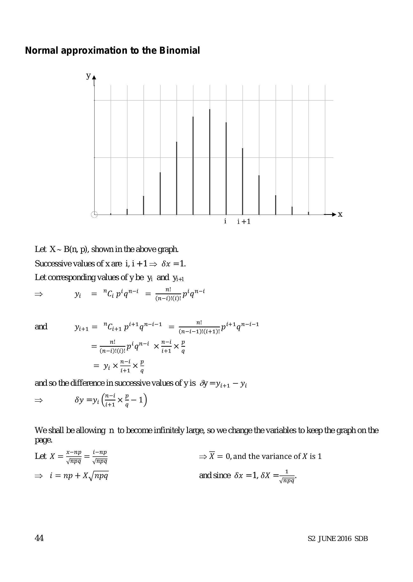
Normal approximation to the Binomialfy yy
iit
Ya
1
Let X~ B(n, p), shown in the above graph.
Successive values of xare i,it+t1l=> 6x =1.
Let corresponding values of y be y, and yi
ar ni oo
=> A = "CG pq” U =- apm 1" U
i -i- n! i -i-
and Vier = "Cia pitt” i-1 =- mopar a" i-1
—__7! ipn-i y Mot
~ mpm? q x itd x q
= nity P
= vi x i+1 x q
and so the difference in successive values of yis dV =yi44 — yi
=> by =yi (x 2-1)
i+1 q
We shall be allowing n to become infinitely large, so we change the variables to keep the graph on the
page.
— *mp _ i-np y_ . .
Let X = = = => X = 0,and the variance of X is 1
_ . _ _ 1
=> i=np+X,/npq and since 6x =1, 6X ae
44 $2 JUNE 2016 SDB
---
Page 47
Extracted Text
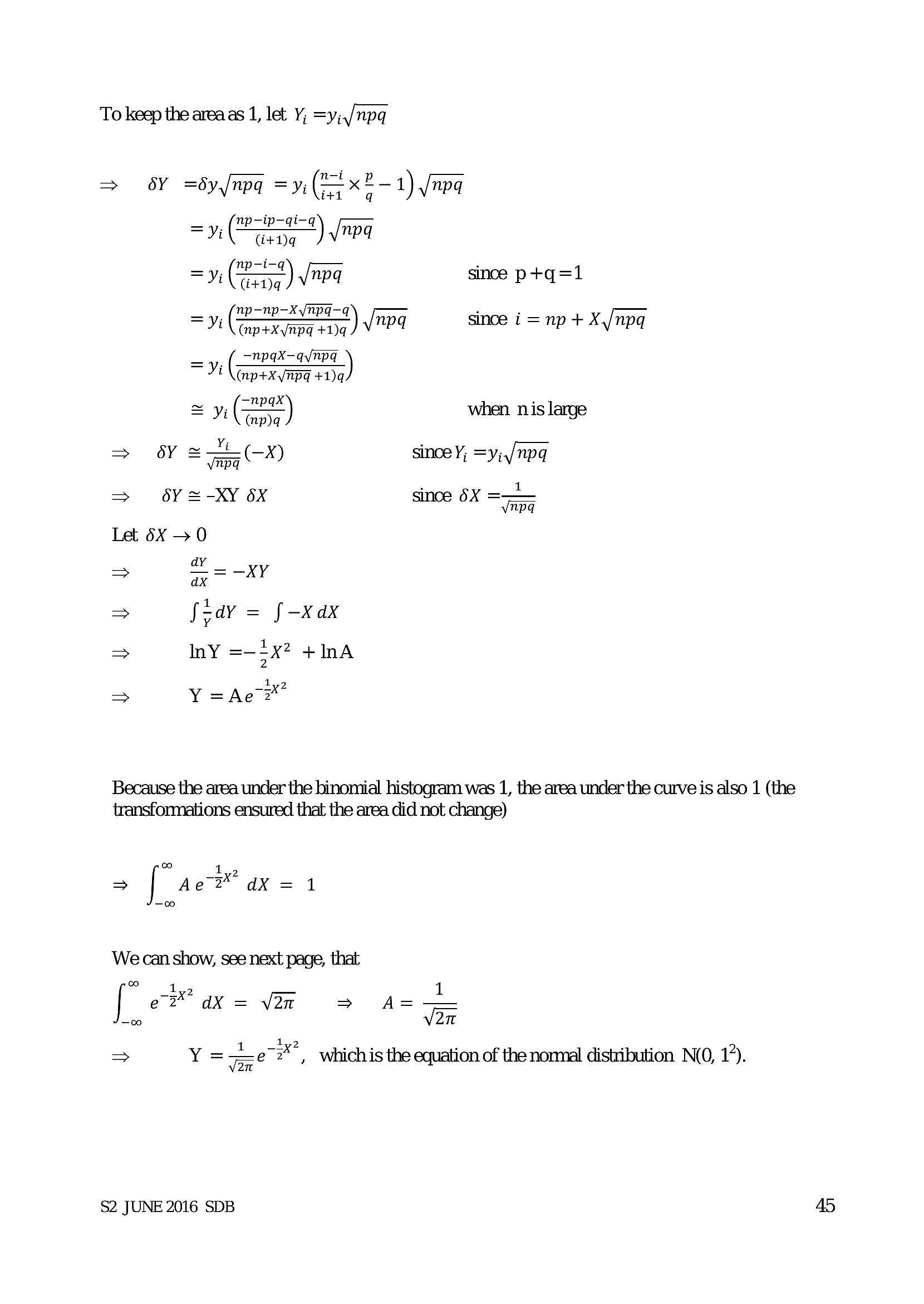
To keep the area as 1, let Y; =y;,/npq6Y =dy/npq = yi ($5 x2—1)./npq
= -ip-qi-q
= y; (ees Gi+Dq ). vine a Jnpq
_ np—-i-q . _
= yi (*) Jaa since p+q=1
_ np—np—X/npq-q . _
= yj a) since i = np + X,/npq
= (eee =npax—avnpg ce)
Ji (np+X/npq +1)q
may, (TMI .
= yi (2S) when nis large
~ Yi : ny
=> oY a X) since Y; =y;,/npq
. 1
> = -XY 6X since 5X Ta
Let 6X > 0
ay
> xT —XY
> fody = f-xdx
=> InY =— 5x? +InA
1
=> Y =Ae2*
Because the area under the binomial histogram was 1, the area under the curve is also 1 (the
transformations ensured that the area did not change)
oo 1
> Ae? dX = 1
We can show, see next page, that
dye 1
e 2° dX = V2n > A=—
[. 20
=> Y =—Le¢"#", whichis the equation of thenonmal distribution N(O, 12).
von
$2 JUNE 2016 SDB
---
Page 48
Extracted Text
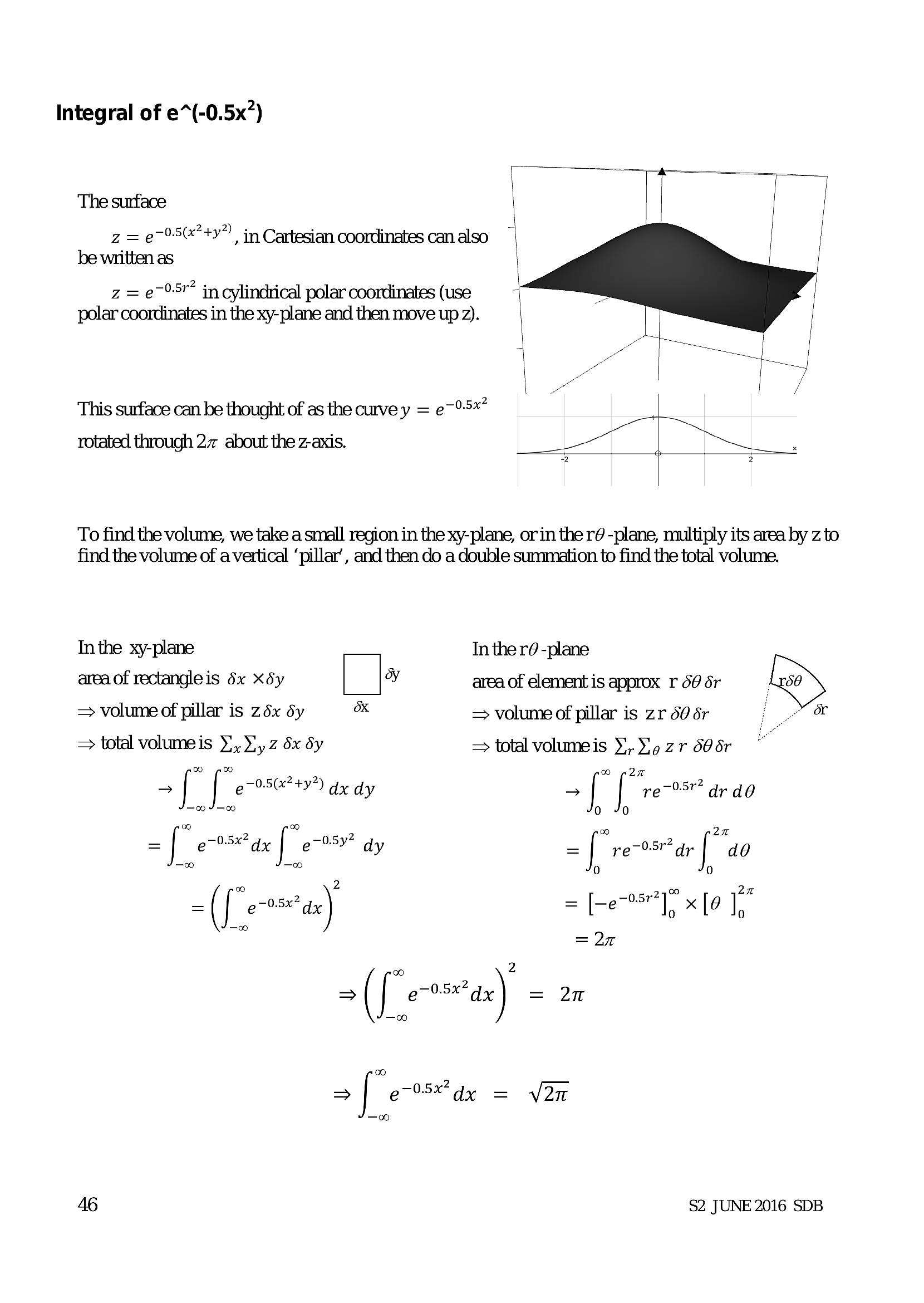
Integral of e*(-0.5x”)The surface
z= e795("+9”) in Cartesian coordinates can also
be written as
z = e~°5" in cylindrical polar coordinates (use
polar coordinates in the xy-plane and then move up 2).
This surface can be thought of as the curve y = e~°-5**
rotated through 27 about the z-axis.
To find the volume, we take a small region in the xy-plane, orin the ré -plane, multiply its area by z to
find the volume of a vertical ‘pillar’, and then do a double summation to find the total volume.
In the xy-plane In the ré -plane
area of rectangle is 6x xdy ¥y area of element is approx r 50 dr
=> volume of pillar is 26x dy ox => voluns of pillar is zr 56 ér i oe
=> total volumeis ¥), Vy z dx dy = total volumeis Y.Yy zr 605r
> [ [ e 7 0-3(x? 4+") dy dy > [ [reo dr de
—09 ¥—0O 0 0
ee) ce) i) 2a
=| eax | e958 dy =| re-osrdr | do
00 0 0 0
«o > 2 -0.5r27% 2n
= | e70-5x" dy = [-e 1, x [0 1,
~ = 27
oo 2
>(J sar) = 2n
={ e095 dy = Vn
46 $2 JUNE 2016 SDB
---
Page 49
Extracted Text
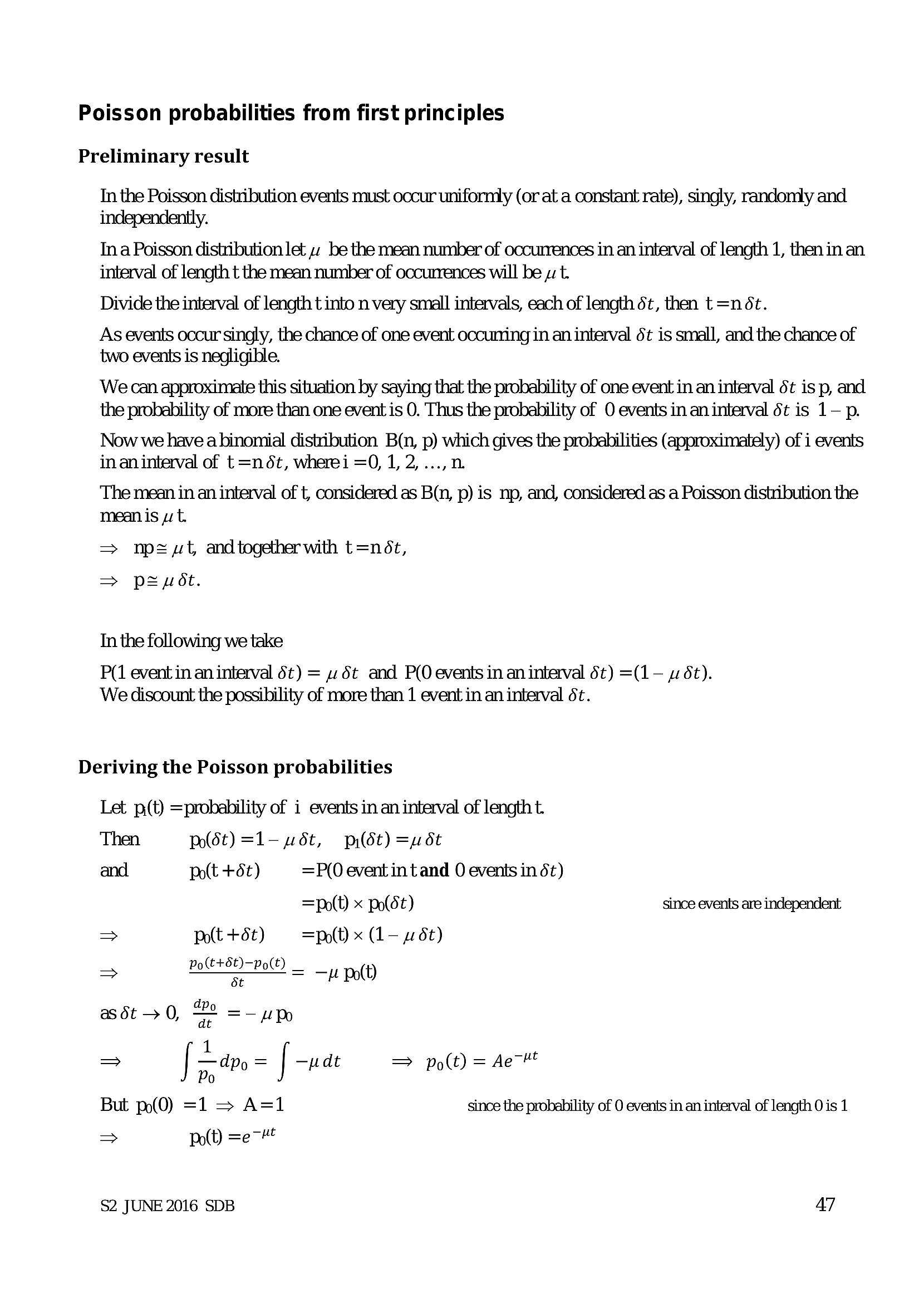
Poisson probabilities from first principlesPreliminary result
In the Poisson distribution events must occur uniformly (or at a constant rate), singly, randomly and
independently.
Ina Poisson distribution let 4 be the mean number of occurrences in an interval of length 1, then in an
interval of length t the mean number of occurrences will be yu t.
Divide the interval of length t into n very small intervals, each of length 6t, then t=n6ét.
As events occur singly, the chance of one event occuring in an interval 6t is small, and the chance of
two events is negligible.
We can approximate this situation by saying that the probability of one event in an interval 5t is p, and
the probability of more than one event is 0. Thus the probability of O events in an interval St is 1— p.
Now we havea binomial distribution B(n, p) which gives the probabilities (approximately) of i events
in aninterval of t =n 6t, wherei =O, 1, 2,...,n.
The mean in an interval of t, considered as B(n, p) is np, and, considered as a Poisson distribution the
mean is zt.
=> npz=wut andtogetherwith t=ndét,
> peut.
In the following we take
P(1 event in an interval 6t) = 2 6t and P(O events in an interval 6t) =(1- ~6t).
We discount the possibility of more than 1 event in an interval St.
Deriving the Poisson probabilities
Let p(t) =probability of i events in an interval of length t.
Then Po(St) =1-6t, pot) =pét
and Polt +6t) =P(0 event int and 0 events in 6t)
=py(t) x po(6t) since events are independent
> Polt +6t) =p(t) x (1- 4 dt)
> oltre po = -u pod)
as dt > 0, Po =— uUPo
1
=> [ -an = [ -wae = po(t) = Ae"
0
But po(0) =1 > A=1 since the probability of 0 events in an interval of length 0 is 1
> Pot) =e"
$2 JUNE 2016 SDB 47
---
Page 50
Extracted Text
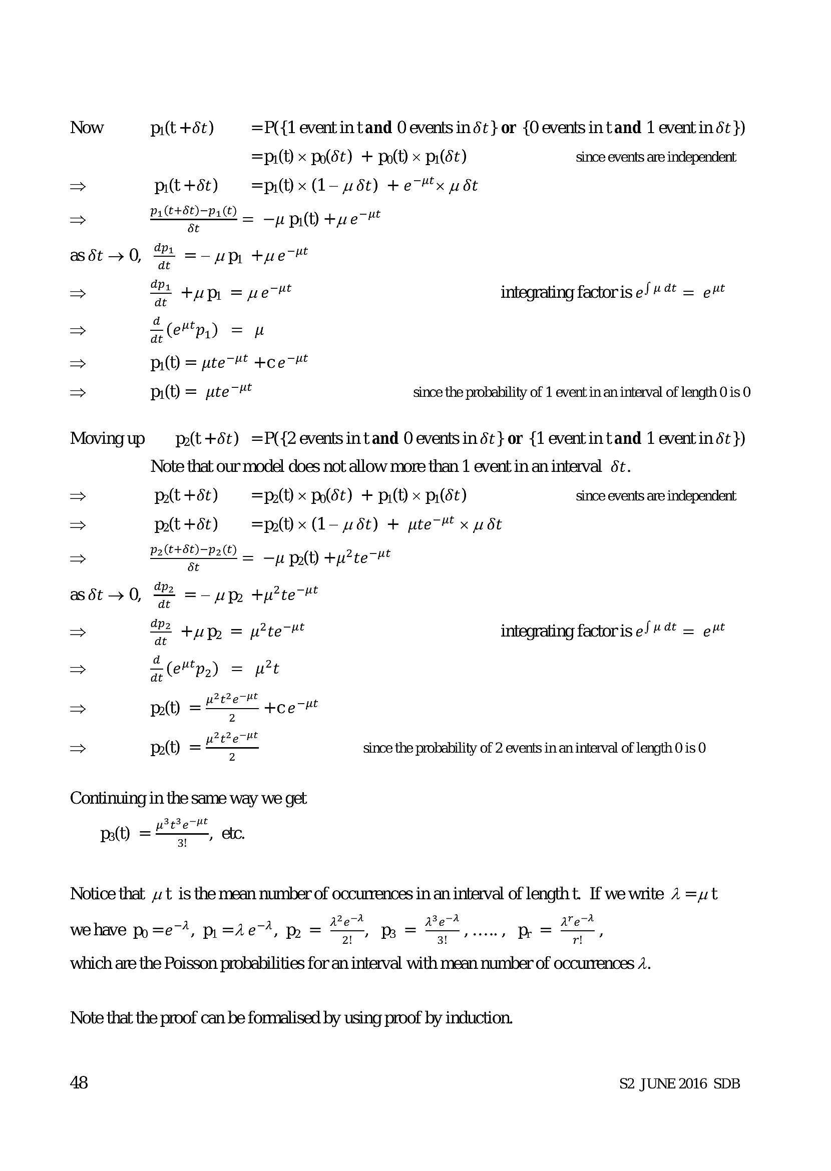
Now pilt +6t) =P({1 event intand 0 events indt} or {0 events intand 1 event in dt })=pi(t) x po(6t) + polt) x pi(St) since events are independent
> pit+ét) =p) (1-wd6t) +e x wot
> paren = —p pit) +we7H
as 6t > 0, oe =-up tue
> oe tupr = pe Ht integrating factoris e/#@t = et
d
5 (eps) =
pit) = pte’ +ce Ht
uuiy
pit) = pte#* since the probability of 1 event in an interval of length 0 is 0
Moving up pot +é6t) =P({2 events intand 0 events in dt} or {1 eventintand 1 event in ét})
Note that our model does not allow more than 1 event in an interval 6t.
> po(t +6t) =pr(t) x po(6t) + pi(t) x pi(6t) since events are independent
> pot +6) =pr(t) x (l- dt) + pte’ x wot
a pire = —p prot) +y2te-#t
as dt > 0, Pe =—"UPo +y?te
> ope +uR2 = w?teM integrating factoris e/"4¢ = ext
=> « (ett) = wt
> p(t) = =“ +ce Ht
> p(t) = _wee since the probability of 2 events in an interval of length 0 is 0
Continuing in the same way we get
pat) <2" ate,
Notice that . t is the mean number of occurrences in an interval of lengtht. If we wnite 2 =ut
qze4 AeA Area
we have Pp =e, pi =Ae, Pp = T— Ps = peeey P=,
3!
which are the Poisson probabilities for an interval with mean number of occurrences 1.
Note that the proof can be formalised by using proof by induction.
48 $2 JUNE 2016 SDB
---
Page 51
Extracted Text
Indexaccuracy, 36
binomial distribution, 6, 14, 23
mean, 9
normal approximation, 23
normal approximation, proof, 44:
poisson approximation, 13
probabilities, 7
proof for np and npq, 42
variance, 9
binomial theorem, 6
binomial coefficients, 6
census, 25
combinations, 5
"C,, 6
properties, 5
continuity correction
normal approx to binomial, 23
normal approx to poisson, 24
continuous uniform distribution, 22
mean, 22
median, 22
proof of formulae for mean and variance, 43
variance, 22
Critical region, 28, 32, 33
factorials, 5
hypothesis test, 28
altemative hypothesis, 28
binomial, critical region, 32
binomial, two-tail, 32
null hypothesis, 28
one-tail, 30
poisson, critical region, 33
poisson, one tail, 33
two-tail, 30
using normal approximation, 34
$2 JUNE 2016 SDB
pascal’s triangle, 6
poisson distribution, 10
conditions, 10
mean, 12
normal approximation, 24
probabilities, 11
probabilities from first principles, 47
variance, 12
population, 25
finite, 25
probability density function
conditions, 15
mean, 19
median, 20
mode, 20
quartiles, 20
variance, 19
sample, 25
advantages, 26
disadvantages, 26
simple random, 25
sampling distribution, 25
worked example, 27
sampling frame, 25
sampling unit, 25
significance level, 28
actual level, 29
binomial, 29
meaning, 28
poission, 29
statistic, 25
test statistic, 28
49
---
Struggling with the concepts in this paper?
Revise syllabus notes, key exam points, and interactive practice questions for Statistics: