Statistics_3_Revision_short_notes

Extracted Content: Statistics_3_Revision_short_notes

Page 1

Extracted Text

Statistics 3

Revision Notes

J une 2016

---

Page 2

Extracted Text

S3 JUNE 2016 SDB

---

Page 3

Extracted Text

Statistics 3

1 Combinations of random variables ............ccsssccssssssscssssssescesssessscsscssssscessssssesesssssessessessesssecesssseseceees 3

3 —_ Biased & unbiased estimator............sssssssosessssssesessessessesssessesessesesessssesessasssssessssssssssssesessesssesesseeseees 8
Unbiased estimators of 1 ado 7 o.ccescsssssscsssssesscssssssssssssssssssssesssssssscsssssssscsssssuscsssssscsssssuecssssssesssssuessssses 11
Estimating sc and o? froma SaMple ......sssssssssssssssssesssssecsssssscsssssccssssscsssssccessuscsssusccessuscessnscsessuscsssssccessuecsssneccessuecessseceessses 11

4 Confidence intervals and significance tests............csscssssssssscsssescsssessssessssescssescssssssessessceeees 14
Sampling istrilbution Of the MOAN... eesesesssesessseseseceseseceseseceseseceseseceseseseseseceseseseseseseseseseseseaeseseseseses 14
Central limit theoremand standard Erin ..........ecsssssscecsssscececsesssesscseseeesscseenssesesecucesscsecusssscscnessaceeeneasens 15
Confidence intervals «0.0.0... ssessssesssssscsecnssssesecssssscccussesesecussssecscsesesusscsesneusscseaneusscsecnsesscscnssssesecneseaseneneasees 16
Central Limit Theorem Example ....ssssccssssssssssssssssssssssssssssssssssssssssssssssssssssssssssssssssssusssssssssssssessssuuunssssssssssseessusuuesssseesees 16
Significance testing- variance of population known 18
Mean of normal Gistribution 0... eeceseesessessessseeseseeseseeseseesessesessesessesesscsesucsessesessesessesesseaesueseseeaeseaeseeaeseeseseeaeaeeaeseeaeaeeaeaeaee 18
Difference between means of normal Cistributions ..........eccecesececseceeseeeseeeeseescseescseseseseseeseseeaeeeaeseeaeseeaeseeaeaeeaeseeaeeeeaeeeaee 19
Significance testing - variance of population NOT known, large sample... sseeesseseseeeeseseeeeesseseeeenees 21
Mean of normal Gistribution 0... eeceseesessessessseeseseeseseeseseesessesessesessesesscsesucsessesessesessesesseaesueseseeaeseaeseeaeseeseseeaeaeeaeseeaeaeeaeaeaee 21
Trmmportant ASSUIMHiON «0... eeeesesesesseseesesesessesessesesscsessesessesessesessesessesessesesucsessesesueaesueseseesesucseseaesueaescaesecaeseeaeaeeaeseeaeeeeaeeeeaee 21

---

Page 4

Extracted Text

5

Spearman’ s rank conelation coefficient.

Comparison between PMCC and Speanman..........ssscessecsssecsssecesecsesecsesecsesecsesecsesecsesecsesecsesecaesecaesecaeaecaeseceeaeeaeaeeaeaeeaeaeeaeaeeed 32
7 APPeENdix......rccccocscceseccseseccsesecssssecsseseesssseessssessssseesseseessesessseseecsssesssesesssssescsesescessesssssesssesesessseecesseseeee 33

Combining random variables 0.0.00... cceesssessssssessscsesssceeseseneeseeseeseeseseseseeeesceeseeeeeeeteeeseeeeeetseeeenseeeees 33
EDX FY] = EDX] HEY) oe eeseeceecseesseesessesseessecssecscessecssccasesucessecsecacesseeasecaesseesuecaasueesseeaasaeesueeasecaeesueeseeeaeecaeeneeaeeeseensees 33
VarlX FY] = VarkX] FV aly) one eeceeceecseecseesseessecseecseesseessecssesseessecasecseesseessecueesueessecaeesueesuecasesueesueesuecaeesseeseeeaeenseenseeaseseed 34

Unbiased & biased eStirAtors...... ce ecesessseseseseseseseseseseseneseseseseseseseseseseseseseseseseseseseseseseseseseseseseseseseseaesens 34
Unbiased estimators ...

Biased Estimators

Unbiased estimates of population mean and VariANCe.......eseesesesesesesesesesesesesesesescsesesesesesesesesesesesesenesens 35
Unbiased estimate of the mean.

Probability generating fUNCHOMS «00... eeeeseseeeetceetsecteeceseceseeesessesceesceeseeeesteteteeesestetetstetseseeeees 39
Expected mean and variance for a p.G.f.......secsssscsssscsssecsesecsesecsesecsesesseseesesecsesecsesecsesecseaecsesecaesecaesecaeaecaesecaeseeaeaeeaeaeeaeaeeeeaeeed 39
Mean and variance of a Binomial distribution
Mean and variance of a Poisson distribution.

TNdeX.......sssosessssssesecsscssesssssssnsssssssensssssscenssssescensseseseesssesessssessessseseeesssesesnsssesensssssessssssssssessssesessesessssseeeess

2 S3 JUNE 2016 SDB

---

Page 5

Extracted Text

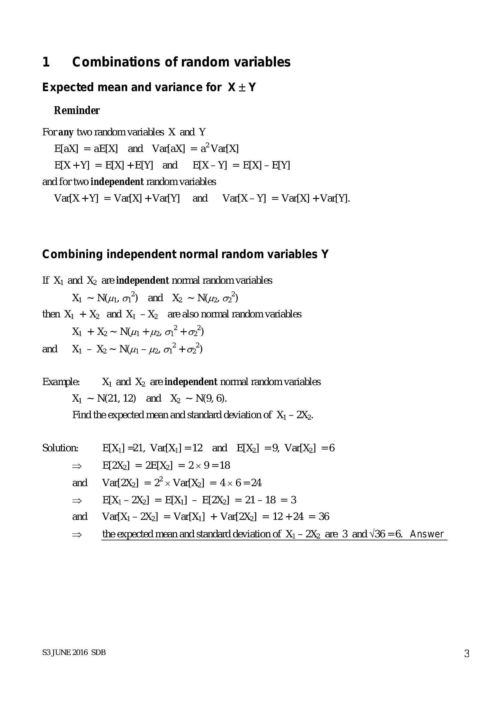
1 Combinations of random variables Expected mean and variance for X+Y

Reminder

Forany two random variables X and Y
E[aX] = aH[X] and VarfaX] = a’Var{X]
E[X +Y] = E[X]+E[Y] and E[X-Y] = E[X]- EY]
and for two independent random variables
Va{X+Y] = Vat{X]+Va{Y] and ValX-Y] = Va{X] +VatyYl.

Combining independent normal random variables Y

If X; and X2 areindependent nonnal random variables
X1 ~N, or) and X ~ Niwa, 07’)

then X; +X) and X; -X» arealso normal random variables
X + Xo ~ Nia tyn, oF +o’)

and X - Xo~ Nun - wy, of +o’)

Example: X, and X2 areindependent nonnal random variables
X ~N(21,12) and X% ~NQ, 0.
Find the expected mean and standard deviation of X; - 2X.

Solution: EX] =21, VatX] =12 and E[X)] =9, VatX] =6
> E[2X2] = 2E[X%)] = 2x 9=18
and = Var{2X2] = 22x Var{X:] = 4x 6 =24
=> E[X - 2X2] = EDX] - E[2X,] = 21-18 =3
and = Var{Xy- 2X2] = Var[Xi] + Varl2X)] = 12 +24 = 36
> the expected mean and standard deviation of X;- 2X2 are 3 andV¥36 =6. Answer

S3 JUNE 2016 SDB

---

Page 6

Extracted Text

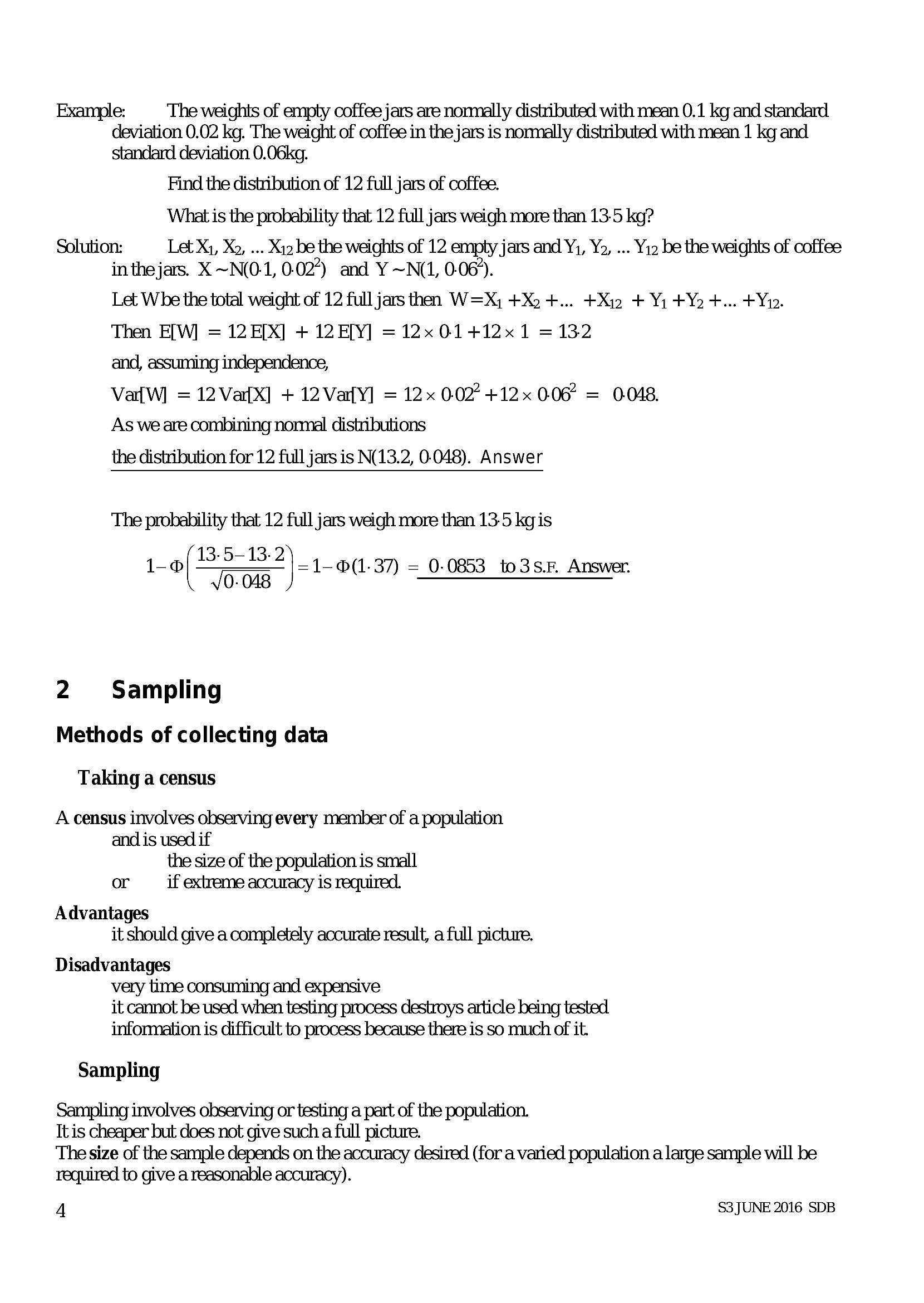
Example: The weights of empty coffee jars are nonmally distributed with mean 0.1 kg and standard deviation 0.02 kg. The weight of coffee in the jars is normally distributed with mean 1 kg and standard deviation 0.06kg.

Find the distribution of 12 full jars of coffee.
What is the probability that 12 full jars weigh more than 13-5 kg?

Solution: Let Xi, Xo, ... X12 be the weights of 12 empty jars and Y;, Yo, ... Yi2 be the weights of coffee
inthejars. X ~N(0-1, 0-02) and Y ~N(1, 0-064.

Let Whe the total weight of 12 full jars then W=X; +X +... +X + Y+¥Yo +... #¥p.
Then E[W] = 12 E[X] + 12 EY] = 12x014+12x1 = 132

and, assuming independence,

VatW] = 12 Va{X] + 12 ValY] = 12x 0.027 +12x 006 = 0048.

As we are combining nommal distributions

the distribution for 12 full jars is N(13.2, 0-048). Answer

The probability that 12 full jars weigh more than 135 kgis
, o( B32

\-1 @(1-37) = 0-0853 to3s.h Answer.
0-048 TTT

2 Sampling
Methods of collecting data

Taking a census

A census involves observing every member of a population

and is used if

the size of the population is small

or if extreme accuracy is required.
Advantages

it should give a completely accurate result, a full picture.
Disadvantages

very time consuming and expensive

it cannot be used when testing process destroys article being tested

information is difficult to process because there is so much of it.

Sampling

Sampling involves observing or testing a part of the population.

Itis cheaper but does not give such a full picture.

The size of the sample depends on the accuracy desired (for a varied population a large sample will be
required to give a reasonable accuracy).

4 S3 JUNE 2016 SDB

---

Page 7

Extracted Text

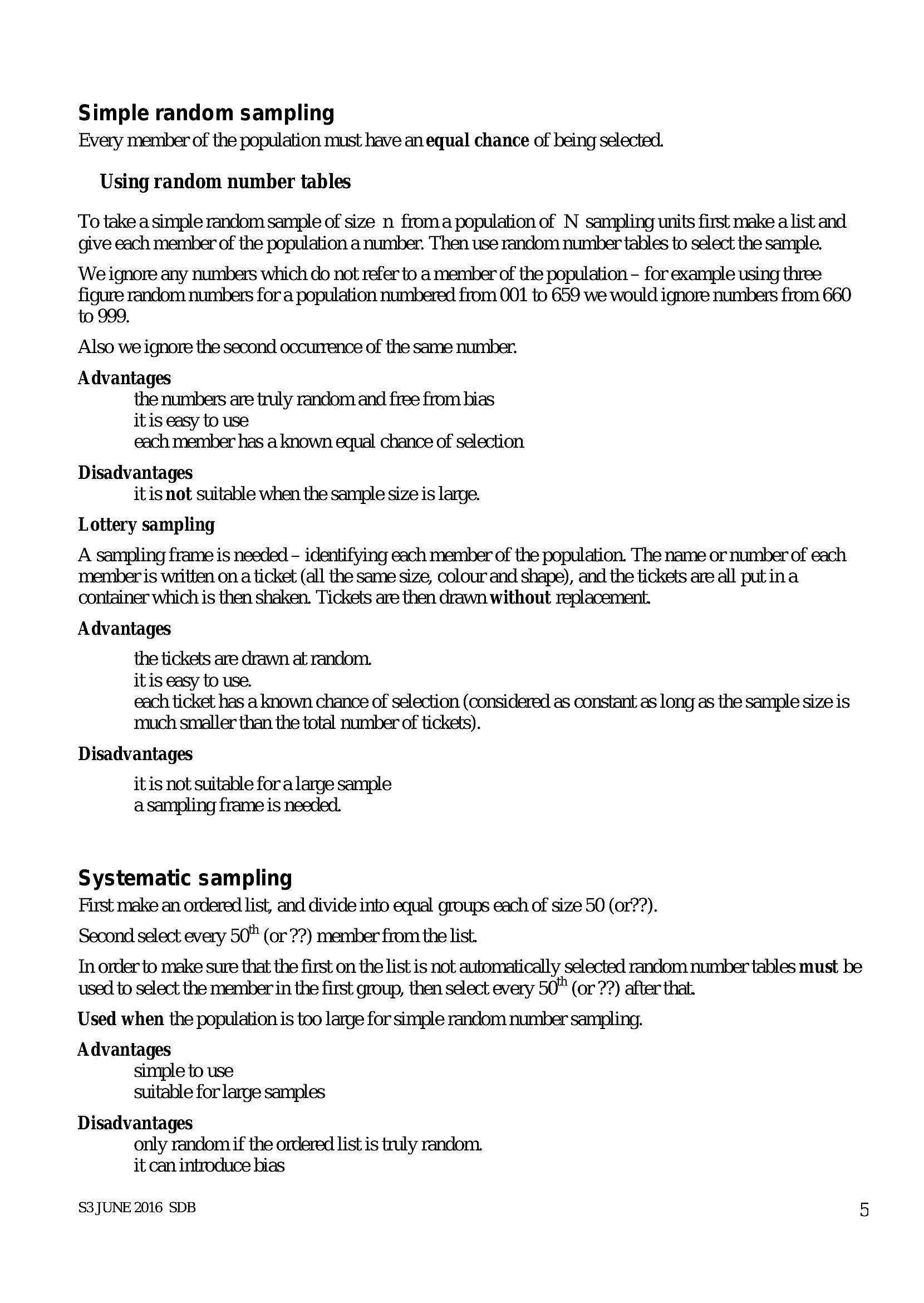
Simple random sampling Every member of the population must have an equal chance of being selected.

Using random number tables

To take a simple random sample of size n froma population of N sampling units first make a list and
give each member of the population a number. Then use random number tables to select the sample.

We ignore any numbers which do not refer to a member of the population - for example using three
figure random numbers for a population numbered from 001 to 659 we would ignore numbers from 660
to 999.

Also we ignore the second occurrence of the same number.

Advantages

the numbers are truly random and free from bias

itis easy to use

each member has a known equal chance of selection
Disadvantages

itis not suitable when the sample size is large.
Lottery sampling
A sampling frame is needed - identifying each member of the population. The name or number of each
member is written on a ticket (all the same size, colour and shape), and the tickets are all put ina
container which is then shaken. Tickets are then drawn without replacement.

Advantages

the tickets are drawn at random.
itis easy to use.
each ticket has a known chance of selection (considered as constant as long as the sample size is
much smaller than the total number of tickets).
Disadvantages

itis not suitable for a large sample
asampling frame is needed.

Systematic sampling
First make an ordered list, and divide into equal groups each of size 50 (or??).
Second select every 50" (or ??) member from the list.
In order to make sure that the first on the list is not automatically selected random number tables must be
used to select the member in the first group, then select every 50" (or ??) after that.
Used when the population is too large for simple random number sampling.
Advantages
simple to use
suitable for large samples

Disadvantages
only random if the ordered list is truly random.
it can introduce bias

S3 JUNE 2016 SDB 5

---

Page 8

Extracted Text

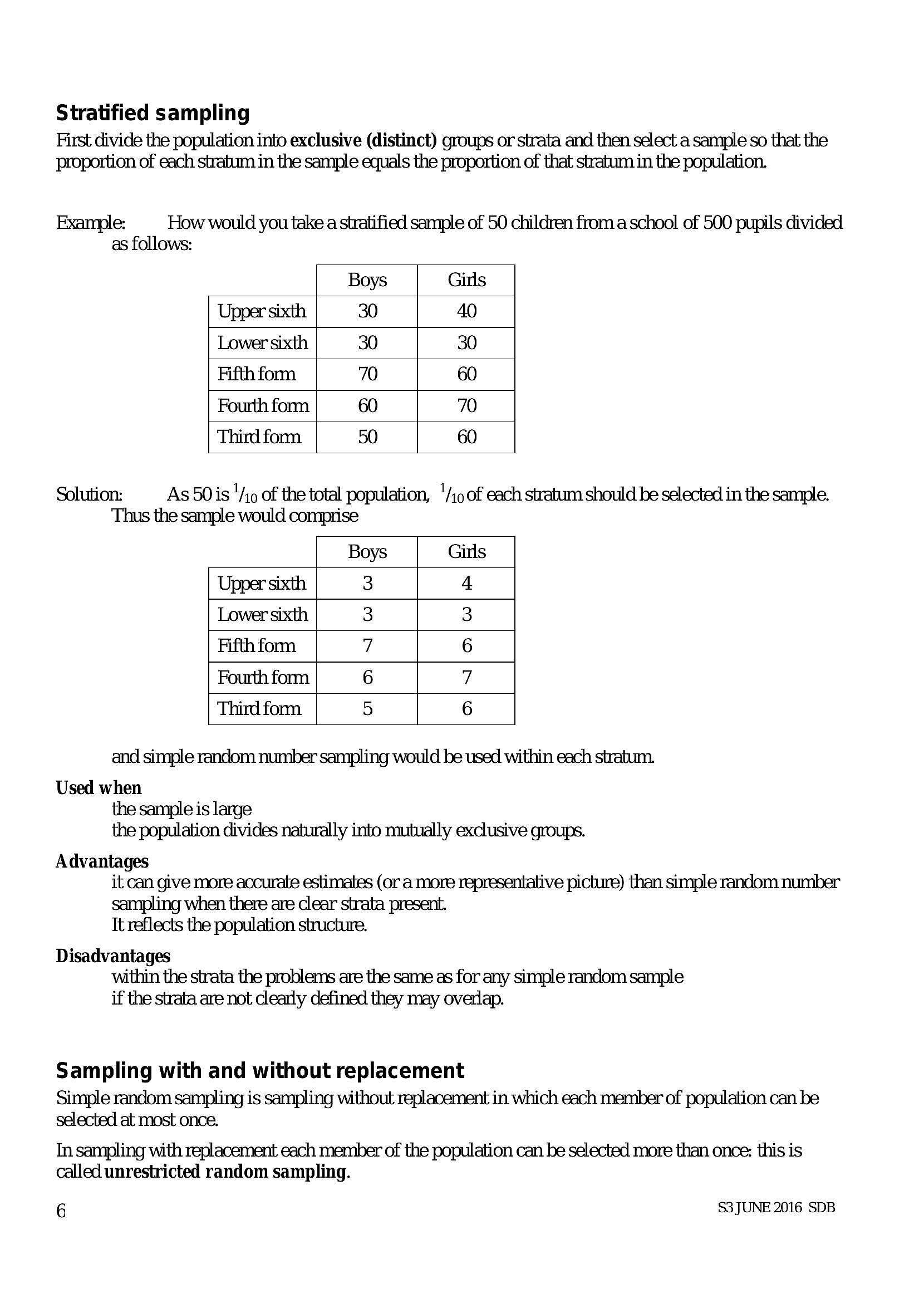
Stratified sampling

First divide the population into exclusive (distinct) groups or strata and then select a sample so that the
proportion of each stratum in the sample equals the proportion of that stratum in the population.

Example: How would you take a stratified sample of 50 children from a school of 500 pupils divided

as follows:
Boys Girls
Upper sixth 30 40
Lower sixth 30 30
Fifth form 70 60
Fourth fom 60 70
Third form 50 60

Solution: As 50 is 1/10 of the total population, 1/19 of each stratum should be selected in the sample.

Thus the sample would comprise
Boys Girls
Upper sixth 3 4
Lower sixth 3 3
Fifth fom 7 6
Fourth fom 6 7
Third fom 5 6

and simple random number sampling would be used within each stratum.

Used when
the sample is large
the population divides naturally into mutually exclusive groups.
Advantages
it can give more accurate estimates (or a more representative picture) than simple random number
sampling when there are clear strata present.
It reflects the population structure.

Disadvantages
within the strata the problems are the same as for any simple random sample
if the strata are not clearly defined they may overlap.

Sampling with and without replacement

Simple random sampling is sampling without replacement in which each member of population can be
selected at most once.

In sampling with replacement each member of the population can be selected more than once: this is
called unrestricted random sampling.

6 S3 JUNE 2016 SDB

---

Page 9

Extracted Text

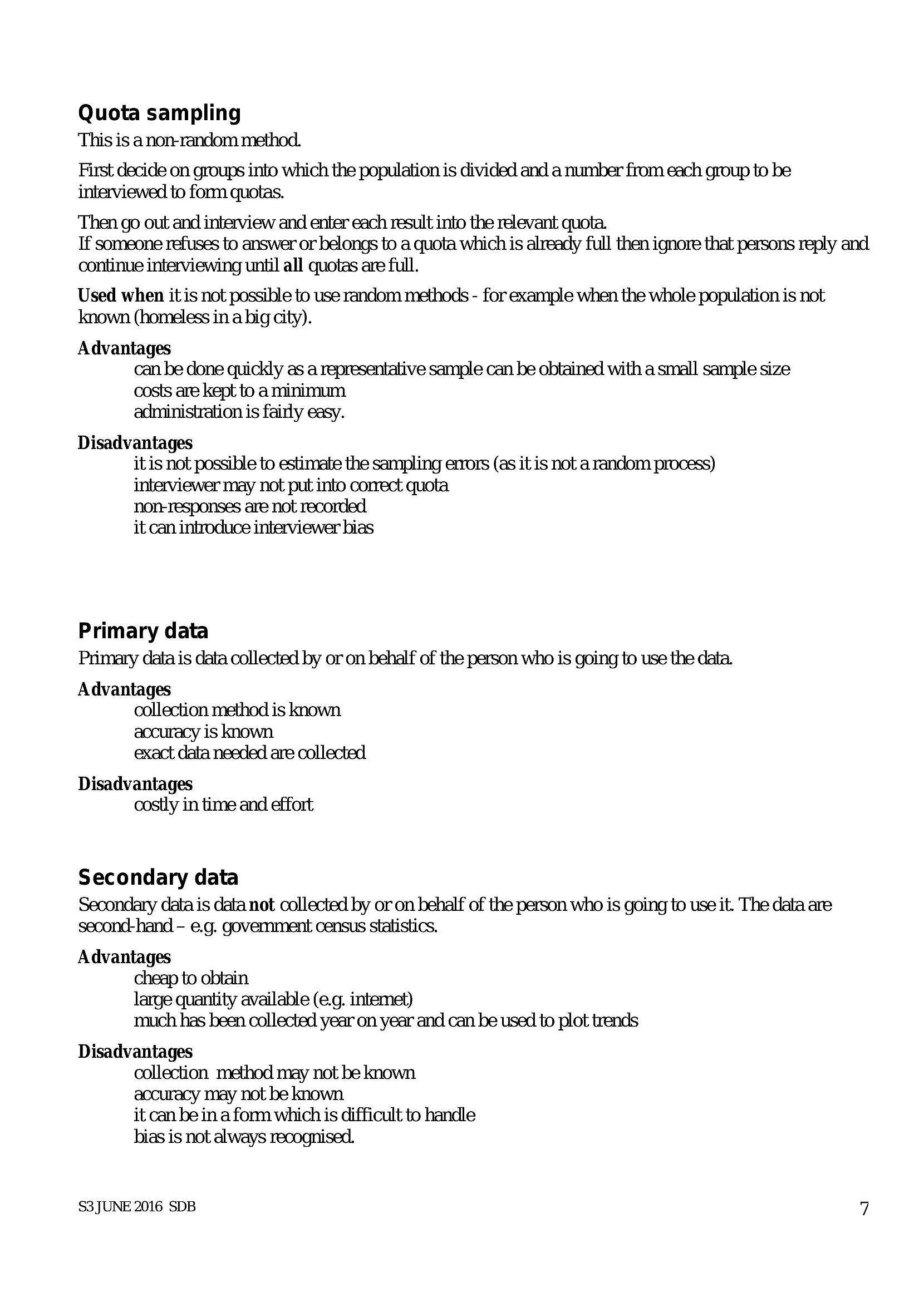
Quota sampling This is anon-random method.

First decide on groups into which the population is divided and a number from each group to be
interviewed to form quotas.

Then go out and interview and enter each result into the relevant quota.

If someone refuses to answer or belongs to a quota which is already full then ignore that persons reply and
continue interviewing until all quotas are full.

Used when it is not possible to use random methods - for example when the whole population is not
known (homeless in a big city).

Advantages
can be done quickly as a representative sample can be obtained with a small sample size
costs are kept to a minimum
administration is fairly easy.
Disadvantages
itis not possible to estimate the sampling emors (as it is not a random process)
interviewer may not put into correct quota
nor-responses are not recorded
it can introduce interviewer bias

Primary data
Primary data is data collected by or on behalf of the person who is going to use the data.
Advantages

collection method is known

accuracy is known

exact data needed are collected

Disadvantages
costly in time and effort

Secondary data

Secondary data is data not collected by or on behalf of the person who is going to use it. The data are
second-hand - e.g. government census statistics.

Advantages

cheap to obtain

large quantity available (e.g. intemet)

mutch has been collected year on year and can be used to plot trends
Disadvantages

collection method may not be known

accuracy may not be known
it can be in a form which is difficult to handle

bias is not always recognised.

S3 JUNE 2016 SDB 7

---

Page 10

Extracted Text

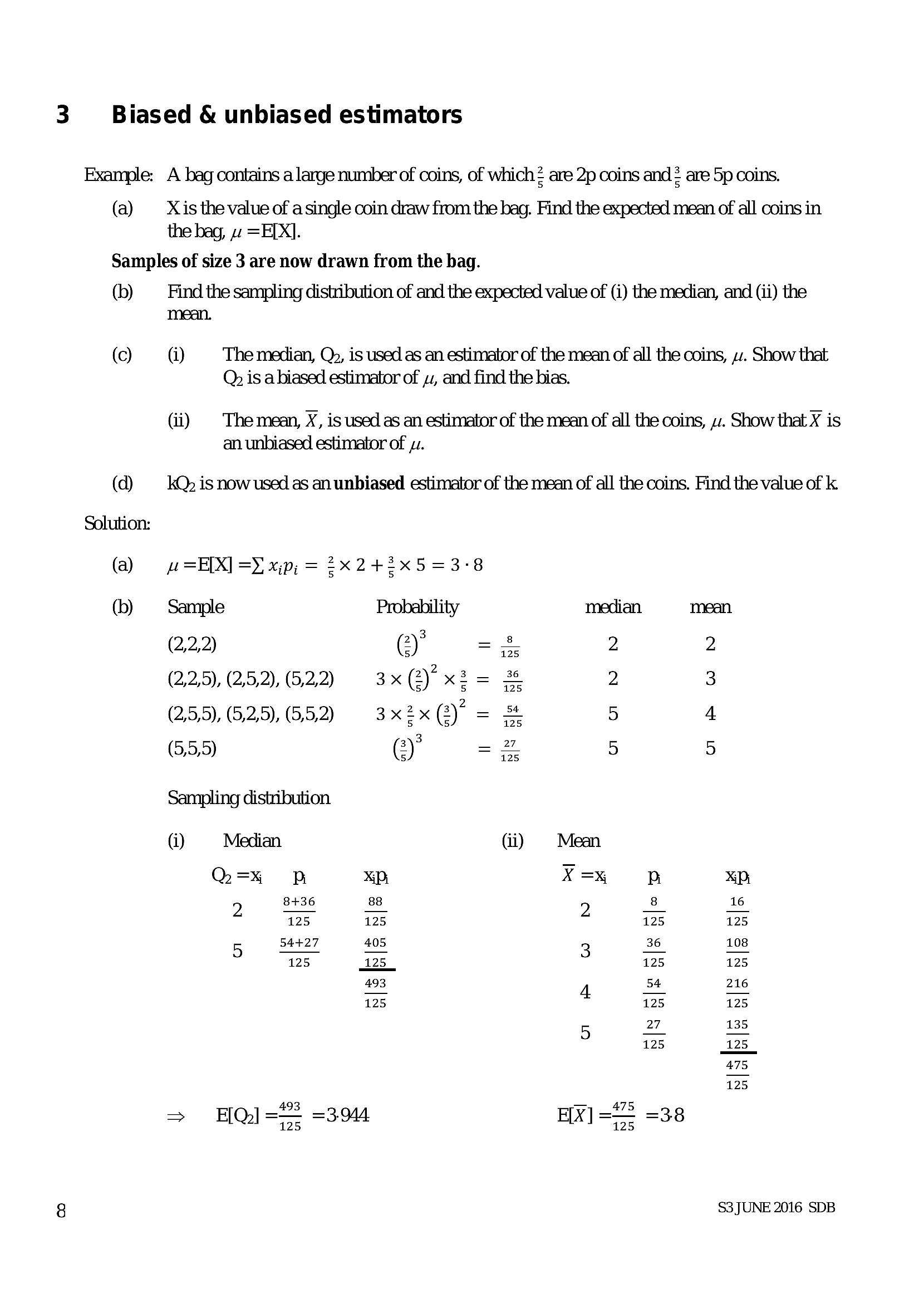
3 + Biased & unbiased estimators

Example: A bag contains a larye number of coins, of which 2 are 2p coins and 2 are 5p coins.

(a) Xisthevalue of asingle coin draw from the bag. Find the expected mean of all coins in
the bag, « =E[X].

Samples of size 3 are now drawn from the bag.

(b) Find the sampling distribution of and the expected value of (i) the median, and (ii) the
mean.

(c) (i) The median, Q», is used as an estimator of the mean of all the coins, zz. Show that
Q is a biased estimator of sz, and find the bias.

(ii) | Themean, X, is used as an estimator of the mean of all the coins, 4. Show that X is
an unbiased estimator of yu.

(d) kQ> is now used as an unbiased estimator of the mean of all the coins. Find the value of k.
Solution:

(a) w=EIX] =) xp, = 2X 24+2x5=3-8

(b) Sample Probability median mean
3
(2,2,2) (2) = is 2 2
(2,2,5), (25,2), (52,2) 3x(2)xi= 3% 2 3
2
(2,5,5), (5,2,5), (55,2) 3x2x() = & 5 4
3
(5,5,5) (:) = 2 5 5
Sampling distribution
(i) Median (ii) Mean
Q=x% PB SP, X=% PB SP
8+36 88 2 8 16
[25 125 125 125
54427 405 3 36° 108
125 125 125 125
493 4 54 216
125 125 125
27 135
5 Ds 125
475
125
> HQ]=— =3944 E[X] == =38

125 125

8 S3 JUNE 2016 SDB

---

Page 11

Extracted Text

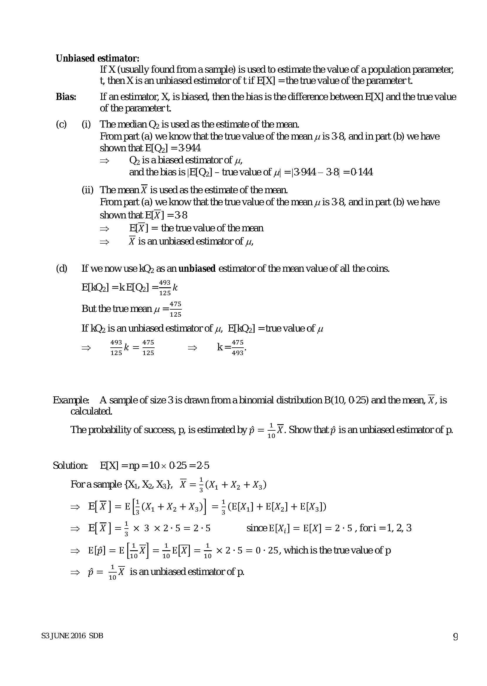
Unbiased estimator: If X (usually found from a sample) is used to estimate the value of a population parameter, t, then X is an unbiased estimator of t if E[X] =the true value of the parameter t. Bias: If an estimator, X, is biased, then the bias is the difference between E[X] and the true value of the parameter t. (c) (i) Themedian Q is used as the estimate of the mean. From part (a) we know that the true value of the mean jis 3-8, and in part (b) we have shown that E[Q.] =3-944 > Q is abiased estimator of 4, and the bias is |E[Qo] - true value of 4 =|3-944 — 3-8) =0-144 (ii) The mean X is used as the estimate of the mean. From part (a) we know that the true value of the mean jis 3-8, and in part (b) we have shown that E[X] =3:8 => E[X] = the truevalueof the mean => X isanunbiased estimator of y,

(d) If wenowuse kQ) as an unbiased estimator of the mean value of all the coins.
493

E[kQo] =KE[Q)] =k

125

But the true mean yz ==

If kQ) is an unbiased estimator of 4, E[kQ2] =true value of wz

493, 475 = «=*75
125. «125 493°

Example: A sample of size 3 is drawn froma binomial distribution B(10, 0-25) and the mean, X, is
calculated.

The probability of success, p, is estimated by 6 = ak. Show that # is an unbiased estimator of p.

Solution: E[X] =np =10x 0.25 =2:5
Forasample {X1, Xo, Xs}, X = 5 (% +X, +X3)
=> E[X]=[=(x, +X, +X3)] = +E] + ELX] + EX)
=> E[X]=;x3x2-5=2°-5 since E[X,] = E[X] = 2-5, fori =1, 2,3

1

E[p] E[=3| =E[X] zy X 2°5 = 0-25, whichis the te value of p

> p= =x is an unbiased estimator of p.

S3 JUNE 2016 SDB fe}

---

Page 12

Extracted Text

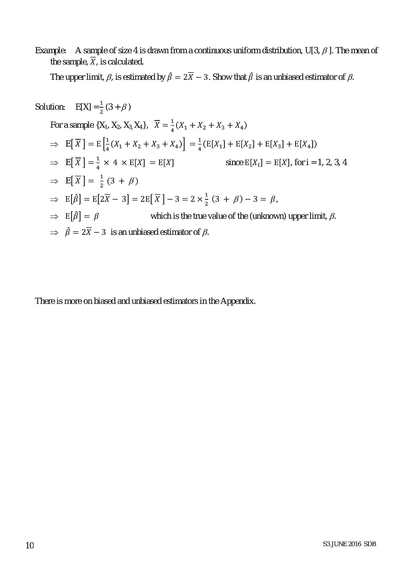
10

Example: A sample of size 4 is drawn froma continuous unifonn distribution, U3, 7 ]. The mean of
the sample, X, is calculated.

The upper limit, 8, is estimated by ? = 2X — 3. Show that # is an unbiased estimator of .

Solution. E[X] => (3 +f)
Fora sample {Xi, Xo, X3.Xa}, K = 2 (X, +X +X3 +X,)
=> E[X]=E[E(x, +X. +X5+X,)] == (EDX) + BLY] + ELX5] + EXD
=> E[X] =; x 4 x E[X] = EX] since E[X;] = E[X], fori =1, 2, 3,4
E[X]= 5G +8)
E[é] = E[2x - 3] = 2E[X]-3=2x>(@ + B)-3=8,
E|[#] = 6 which is the true value of the (unknown) upper limit, /.
B = 2X —3 isanunbiased estimator of £.

Vo Uouvi dv

There is more on biased and unbiased estimators in the Appendix.

S3 JUNE 2016 SDB

---

Page 13

Extracted Text

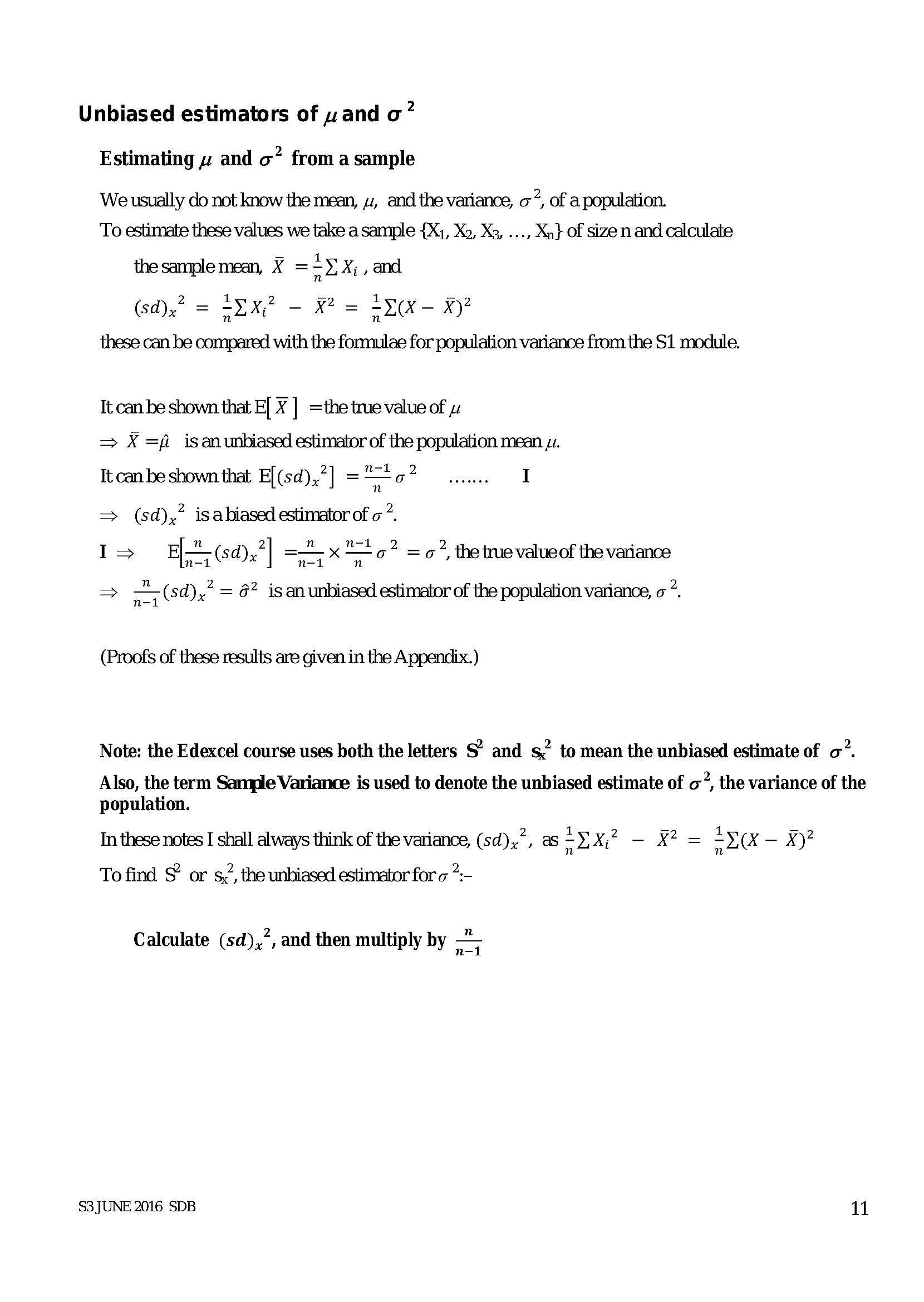
Unbiased estimators of and o” Estimating » and o” from a sample We usually do not know the mean, ., and the variance, ”, of a population. To estimate these values we take a sample {X1, Xo, Xs, ..., Xn} of size n and calculate the sample mean, X ==>% ,and 1

(sd),? = =YX,? - X27 = =yox- x)

n

these can be compared with the formulae for population variance from the S1 module.

It can be shown that E] X | =the true value of wv
= X =f. isanunbiased estimator of the population mean su.

It canbe shown that E[(sd),7] ="=o7 I
=> (sd),” is abiased estimator of o*.
I> EL (sd),"| =x — a? =c7, the true value of the variance

> (sd) = 6? is an unbiased estimator of the population variance, o *.

(Proofs of these results are given in the Appendix.)

Note: the Edexcel course uses both the letters S’ and s, to mean the unbiased estimate of o”.

Also, the term Sample Variance is used to denote the unbiased estimate of o, the variance of the
population.

In these notes I shall always think of the variance, (sd),.”, as =).X;? — X? = =y(x- x)?
To find $ or s2, the unbiased estimator for o 7:-

Calculate (sd),”, and then multiply by a

S3JUNE 2016 SDB al

---

Page 14

Extracted Text

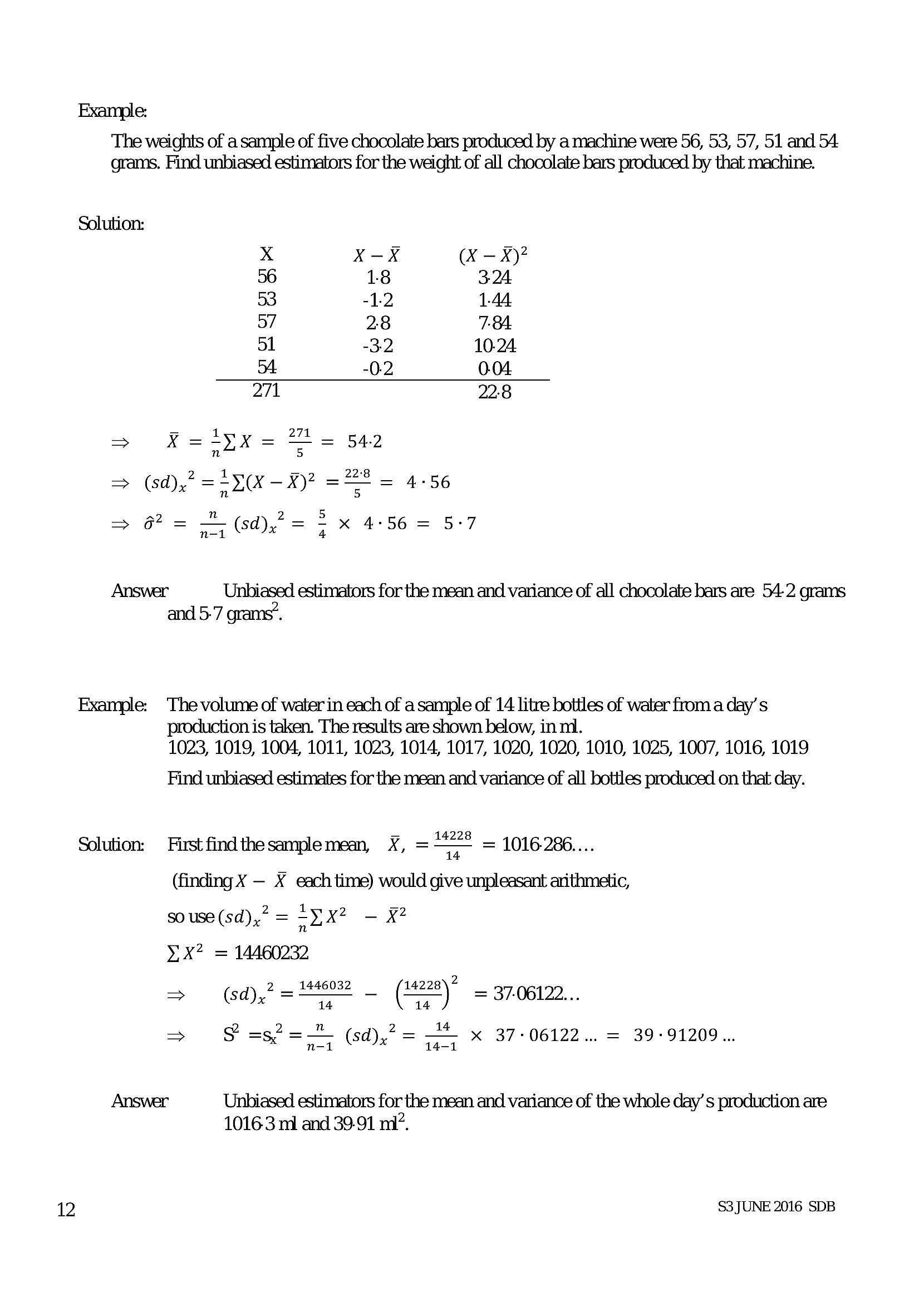
Example:

The weights of a sample of five chocolate bars produced by a machine were 56, 53, 57, 51 and 54
grams. Find unbiased estimators for the weight of all chocolate bars produced by that machine.

Solution:

Xx X-X (X — x)?
56 18 324
53 -1.2 1.44
57 28 7-84
51 -3.2 10-24
54 -0.2 0-04
271 22:8

> 1 271

X =-yX 5 54-2

=> (sd),? = =Y(x — X)? == = 4-56

a2 _ 71 2_ 5 . _ .
fol 1 (sd), 7x 4°56 = 5-7

Answer Unbiased estimators for the mean and variance of all chocolate bars are 54-2 grams

and 5-7 grams”,

Example: The volume of water in each of a sample of 14 litre bottles of water from a day’s
production is taken. The results are shown below, in m1.
1023, 1019, 1004, 1011, 1023, 1014, 1017, 1020, 1020, 1010, 1025, 1007, 1016, 1019

Find unbiased estimates for the mean and variance of all bottles produced on that day.

Solution: Firstfindthesamplemean, ¥, =~““8 = 1016-286...

14
(finding X — X each time) would give unpleasant arithmetic,
souse(sd),? = =yx? — ¥?

n

YX? = 14460232

1446032 14228
> (sd),2= - (

14 14

y = 3706122...

—e2__2 2_ 14 . _ ;
¥ =s2 = (sd)? = 4 x 37-06122... = 3991209...

Answer Unbiased estimators for the mean and variance of the whole day’ s production are
1016-3 ni and 39-91 ni’.

S3 JUNE 2016 SDB

---

Page 15

Extracted Text

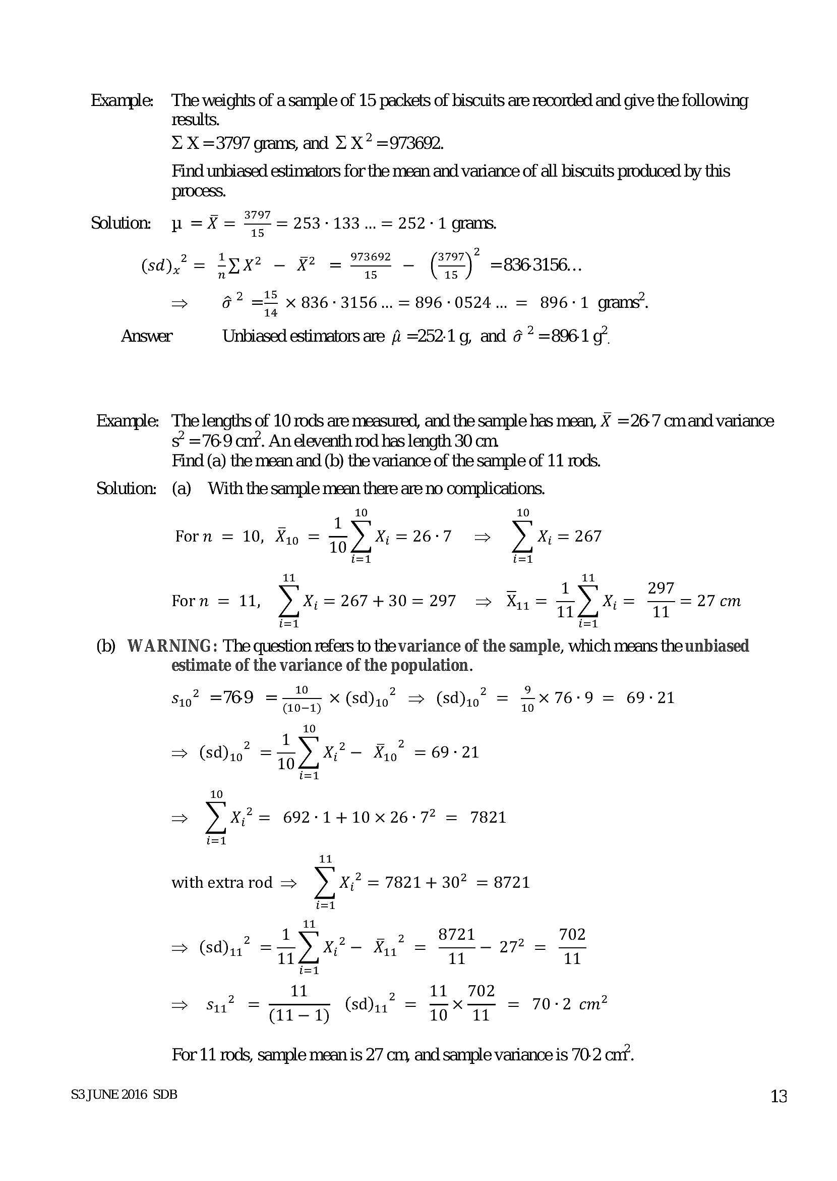
Example: The weights of a sample of 15 packets of biscuits are recorded and give the following results.

= X =3797 grams, and = X? =973602.

Find unbiased estimators for the mean and variance of all biscuits produced by this
process.
> 3797

Solution. p =X = a = 253-133... = 252-1 grams.

2
(sd),? = =x? — x2 = _ (7*)" = 936.3156...

15 15
=> 6? == X 836-3156... = 896-0524... = 896-1 grams’.
Answer Unbiased estimators are =252-1g, and ¢ 7 =896-1 7,

Example: The lengths of 10 rods are measured, and the sample has mean, X =26'7 cmand variance

s’ =76-9 cnt. An deventh rod has length 30 cm
Find (a) the mean and (b) the variance of the sample of 11 rods.

Solution: (a) With the sample mean there are no complications.

1 10 10
Forn = 10, Xi) = aD 26-7 yx 267
i=1 i=1
11 11
_ 1 297
Forn = 11, YX; = 267 + 30 = 297 Xi.= x= = 27cm
La 14 11
= t=

(b) WARNING: The question refers to the variance of the sample, which means the unbiased
estimate of the variance of the population.

10 9
89° =769 = 2 X(sd)io” => (Sd)io” = 5X 76°9 = 69-21

10
1 _
=> (sd)10° =) x= Xp = 69-21
i=1

10
> yixe= 692-1+10x26-7* = 7821
t=1
11

with extra rod = yx? = 7821+ 302 = 8721
i=1

11
1 _ 5 8721 702
= du? =F) X= Ry = = 2 =
i=1
; Way = thy 2 = 70-2 om?
= —— => —x— = .
— Sa = agen 8% = 9% a em

For 11 rods, sample mean is 27 cm, and sample variance is 70-2 cnt.

S3 JUNE 2016 SDB

13

---

Page 16

Extracted Text

4

Confidence intervals and significance tests

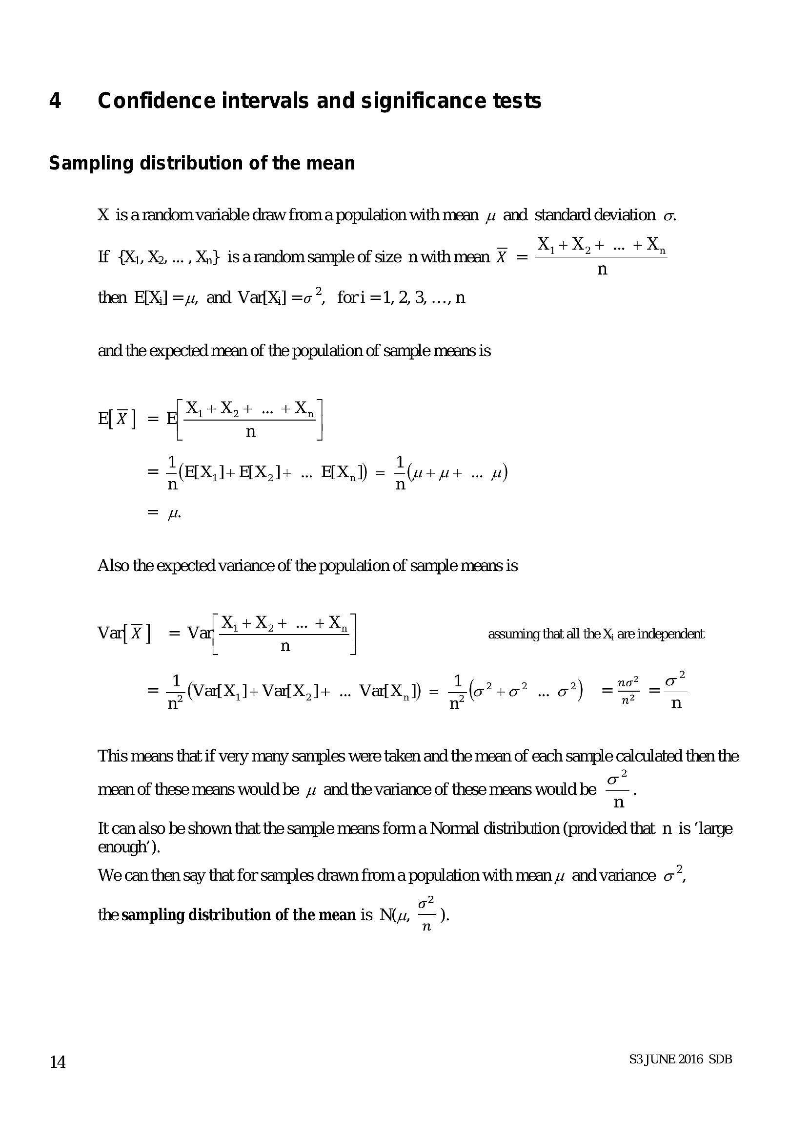
Sampling distribution of the mean

14

X is arandom variable draw froma population with mean 4 and standard deviation o.

. . . = X,+X,+..+X,
If {X1, Xo, ..., Xn} isarandom sample of size nwithmean X = +t

n
then FIX] =, and Vaf{XJ] =o”, fori=1,2,3,...,n
and the expected mean of the population of sample means is
e[X] = pak es +X
n
1 1

= (EDX I+ E[X,]+ ... E[X,]) = quite we fl)
Also the expected variance of the population of sample means is
Var X | = vay ” “%) assuming that all the X; are independent:

= | (atx,]+ Vax Var X 1 (g24g? 92) at ao

= =; (VatX,]+ aX,]+ .. a{X,]) = Sle to? a?) = Tp =

This means that if very many samples were taken and the mean of each sample calculated then the

2

mean of these means would be and the variance of these means would be o.
n

Tt can also be shown that the sample means forma Normal distribution (provided that n is ‘large
enough’).
We can then say that for samples drawn from a population with mean : and variance o?,

2
the sampling distribution of the mean is N(w, — ).

S3 JUNE 2016 SDB

---

Page 17

Extracted Text

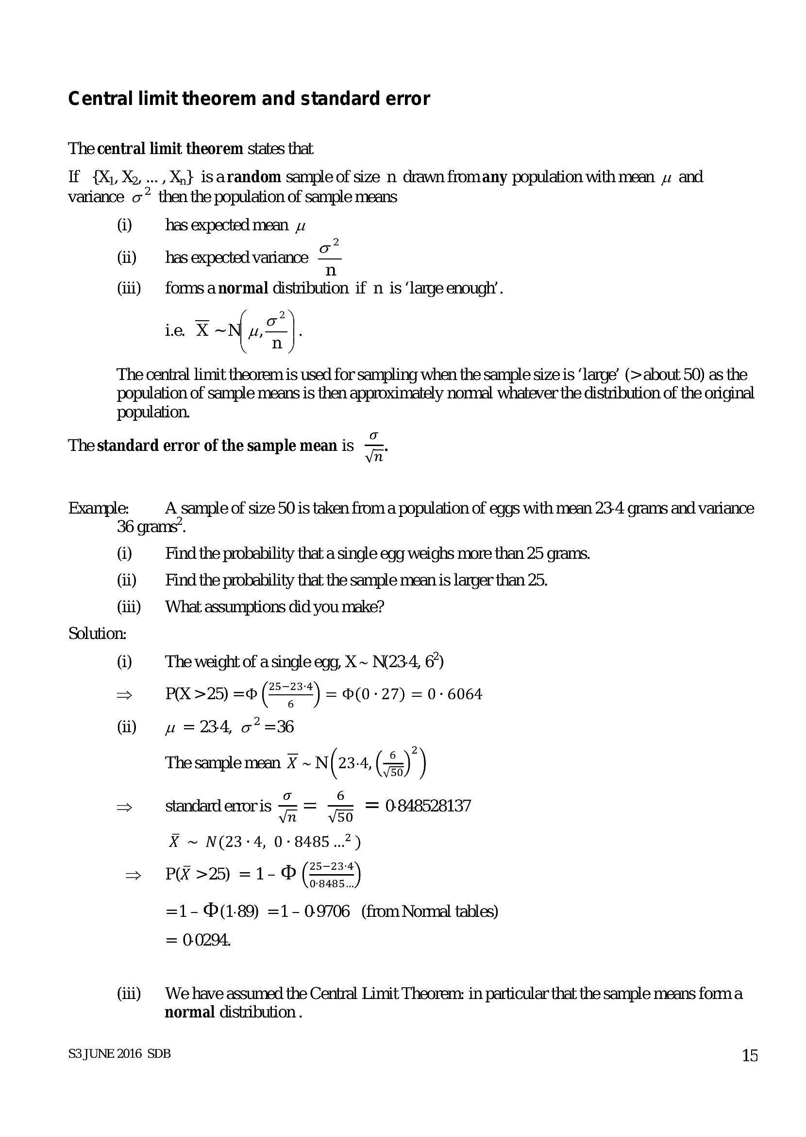
Central limit theorem and standard error

The central limit theorem states that

If {X1, X,..

., Xn} isarandom sample of size n drawn fromany population with mean w and

variance co” then the population of sample means

©)
Gi)

(ii)

has expected mean yu
2
has expected variance a
n
forms anormal distribution if n is ‘large enough’.

_ 2
ie X ~uZ].
n

The central limit theorem is used for sampling when the sample size is ‘large’ (> about 50) as the
population of sample means is then approximately normal whatever the distribution of the original
population.

The standard error of the sample mean is =.

Example:
36
(ji)
(ii)
(iii)

Solution:
(ji)
>

Gi)

(iii)

vn

A sample of size 50 is taken from a population of eggs with mean 23-4 grams and variance

Find the probability that a single egg weighs more than 25 grams.
Find the probability that the sample mean is larger than 25.
What assumptions did you make?

The weight of a single egg, X~ N(23-4, &)
P(X >25) =o (F=*) = (0-27) = 0- 6064
w= 234, 67 =36

The sample mean X ~ N(234, (<))

50.
standard enoris = = — = 0.848528137
vn 50

X ~ N(23-4, 0° 8485..2)
P(X >25) =1- 0(

=)
0-8485...

=1- (1-89) =1- 09706 (from Nonmal tables)
= 0.0294.

We have assumed the Central Limit Theorem: in particular that the sample means fonm a
normal distribution .

S3JUNE 2016 SDB 15

---

Page 18

Extracted Text

Confidence intervals

Central Limit Theorem Example

Example:

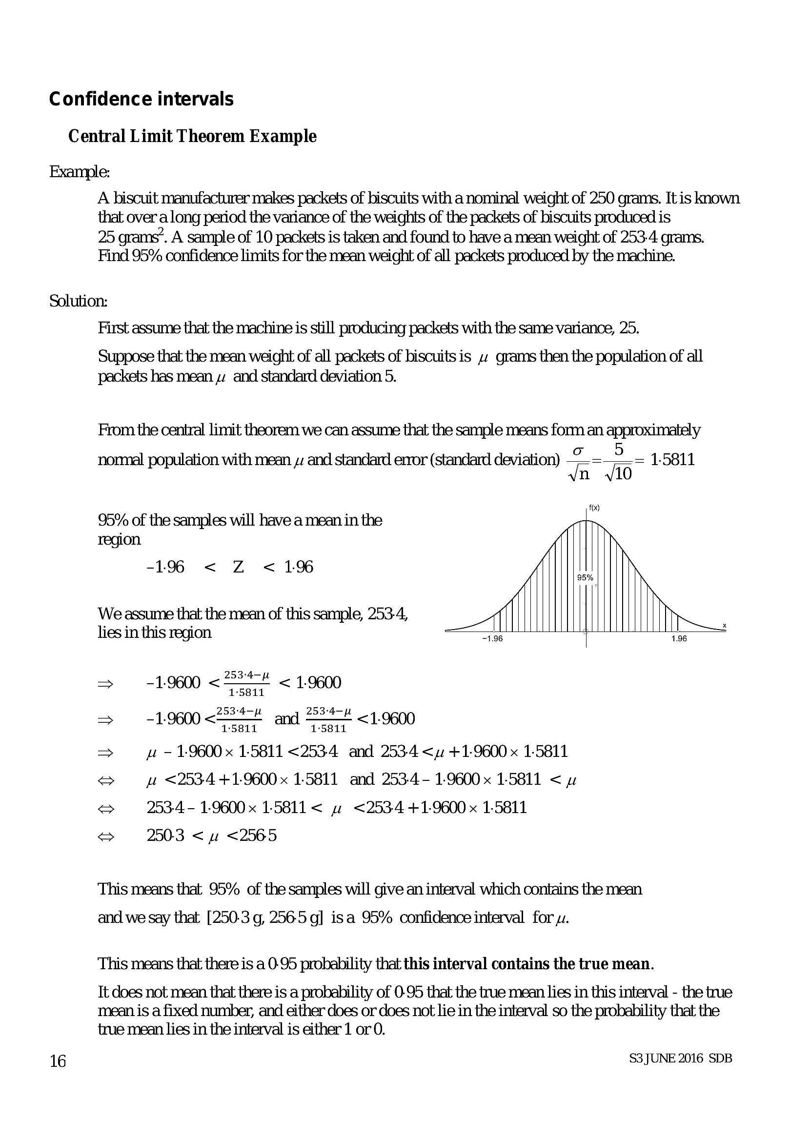
A biscuit manufacturer makes packets of biscuits with a nominal weight of 250 grams. It is known
that over along period the variance of the weights of the packets of biscuits produced is

25 grams’. A sample of 10 packets is taken and found to have a mean weight of 253-4 grams.

Find 95% confidence limits for the mean weight of all packets produced by the machine.

Solution:

16

First assume that the machine is still producing packets with the same variance, 25.

Suppose that the mean weight of all packets of biscuits is 4 grams then the population of all
packets has mean zz and standard deviation 5.

From the central limit theorem we can assume that the sample means form an approximately

nonnal population with mean 4 and standard error (standard deviation) o_8 1.5811

vn 10

fx)

95% of the samples will have a mean in the
region
-196 < Z < 196

We assume that the mean of this sample, 253.4,

lies in this region 88

253-4—p
=> -1.9600 < aoa 1.9600

253-4-p 253-4—p

> ~ 19600 < 15811 15811 <1-9600
> uw - 1-9600 x 1.5811 <2534 and 253-4 <u +1-9600 x 1.5811
S fw <253-4 +1-9600 x 15811 and 253.4- 1-9600 x 15811 < wv
S 253-4. - 1.9600 x 1.5811 < ww <253-4+1-9600 x 1-5811
S 250-3 < uw <2565

This means that 95% of the samples will give an interval which contains the mean
and we say that [250-3 g, 256-5 g] isa 95% confidence interval for yw.

This means that there is a 0-95 probability that this interval contains the true mean.

Tt does not mean that there is a probability of 0-95 that the true mean lies in this interval - the true
mean is a fixed number, and either does or does not lie in the interval so the probability that the
true mean lies in the interval is either 1 or 0.

S3 JUNE 2016 SDB

---

Page 19

Extracted Text

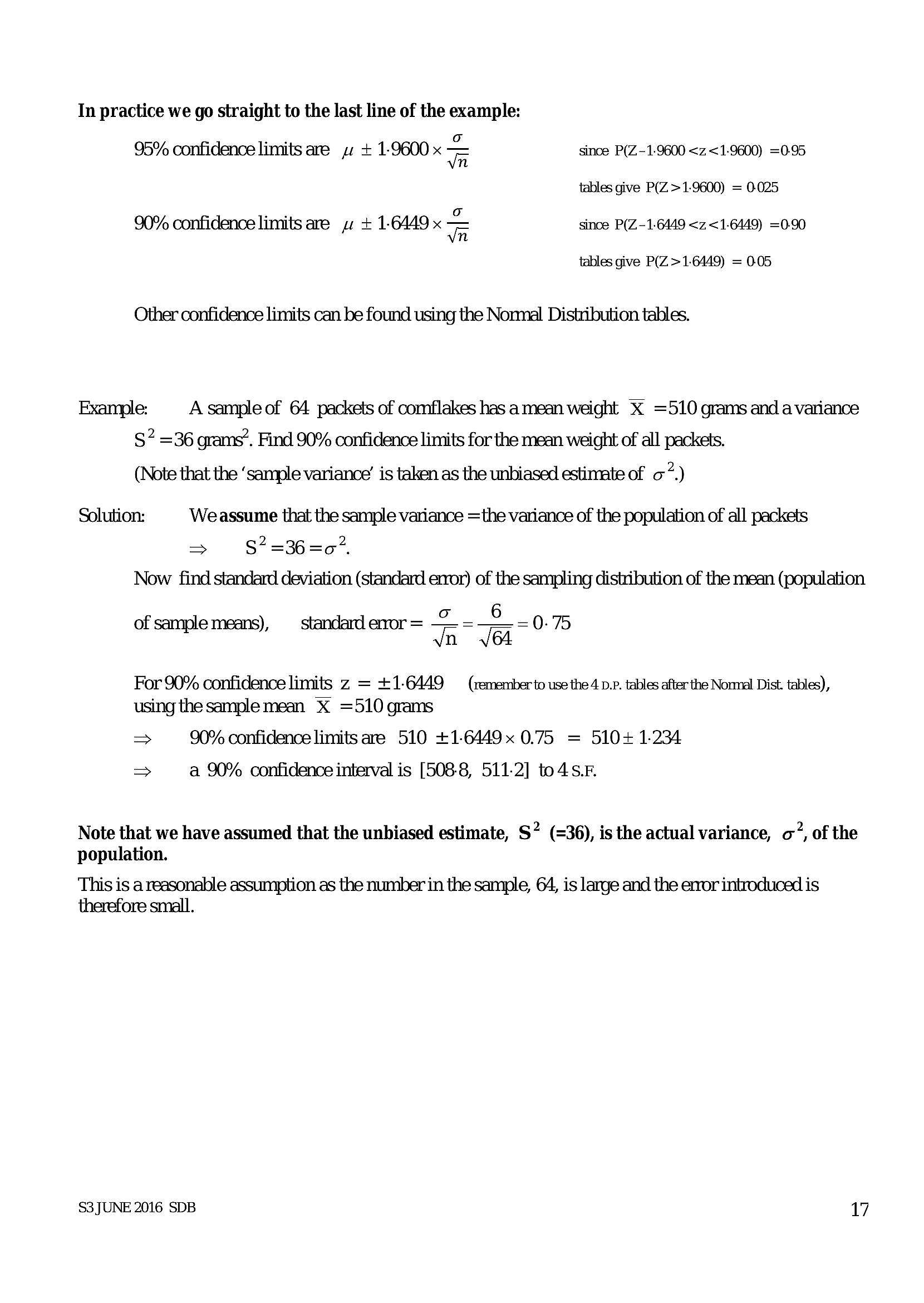
In practice we go straight to the last line of the example:

95% confidence limits are wv + 1-9600 x = since P(Z.~1-9600 <z.<1-9600) =0-95
tables give P(Z>1-9600) = 0025
90% confidence limits are wv + 1-6449 x = since P(Z.-1-6449 <z.<1-6449) =0.90

tables give P(Z >1-6449) = 0.05

Other confidence limits can be found using the Nonnal Distribution tables.

Example: A sample of 64 packets of comflakes has a mean weight X =510 grams and a variance
S” =36 grams”. Find 90% confidence limits for the mean weight of all packets.
(Note that the ‘sample variance’ is taken as the unbiased estimate of a)

Solution: Weassume that the sample variance =the variance of the population of all packets
=> $*=36=07
Now find standard deviation (standard exvor) of the sampling distribution of the mean (population
6

of e means), standard enor = 2. = 2. = 0.75
Sample means) in Ja

For 90% confidence limits z = +1-6449 — (rememberto use the 4 Dp. tables after the Nomml Dist. tables),
using the sample mean X =510 grams

> 90% confidence limits are 510 +1-6449x 0.75 = 510+ 1.234

> a 90% confidence interval is [508-8, 511-2] to4s.F

Note that we have assumed that the unbiased estimate, S? (=36), is the actual variance, o, of the
population.

This is a reasonable assumption as the number in the sample, 64, is large and the error introduced is
therefore small.

S3JUNE 2016 SDB 17

---

Page 20

Extracted Text

Significance testing- variance of population known

Mean of normal distribution

Example:

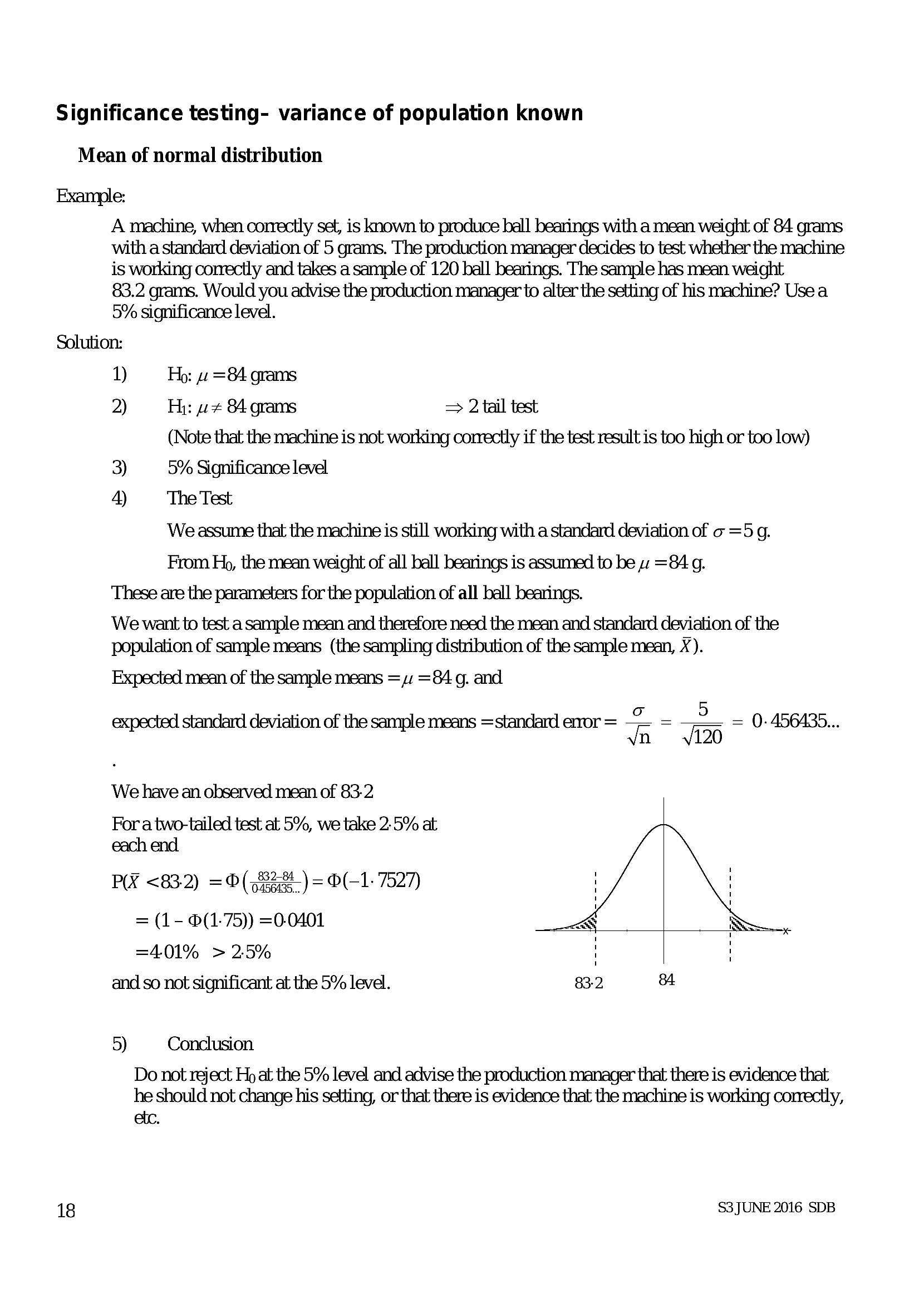
A machine, when correctly set, is known to produce ball bearings with a mean weight of 84 grams
with a standard deviation of 5 grams. The production manager decides to test whether the machine
is working correctly and takes a sample of 120 ball bearings. The sample has mean weight

83.2 grams. Would you advise the production manager to alter the setting of his machine? Use a
5% significance level.

Solution:

18

9) Ho: 4 =84 grams
2) H: wz 84 grams => 2 tail test
(Note that the machine is not working correctly if the test result is too high or too low)
3) 5% Significance level
4) The Test
We assume that the machine is still working with a standard deviation of o =5 g.
From Hp, the mean weight of all ball bearings is assumed to be 4 =84 g.
These are the parameters for the population of all ball bearings.
We want to test a sample mean and therefore need the mean and standard deviation of the
population of sample means (the sampling distribution of the sample mean, X).
Expected mean of the sample means = 4: =84 g. and

expected standard deviation of the sample means =standard exor = i =
n

= 0- 456435...

gle
fan)

We have an observed mean of 83-2

For a two-tailed test at 5%, we take 2.5% at
each end

PR <832) = 0({82:8) = 0(-1- 7527)
= (1- 0(1-75)) =0-0401
=401% > 25%
and so not significant at the 5% level. 83-2 84

5) Conclusion.

Do not reject Ho at the 5% level and advise the production manager that there is evidence that
he should not change his setting, or that there is evidence that the machine is working correctly,
etc.

S3 JUNE 2016 SDB

---

Page 21

Extracted Text

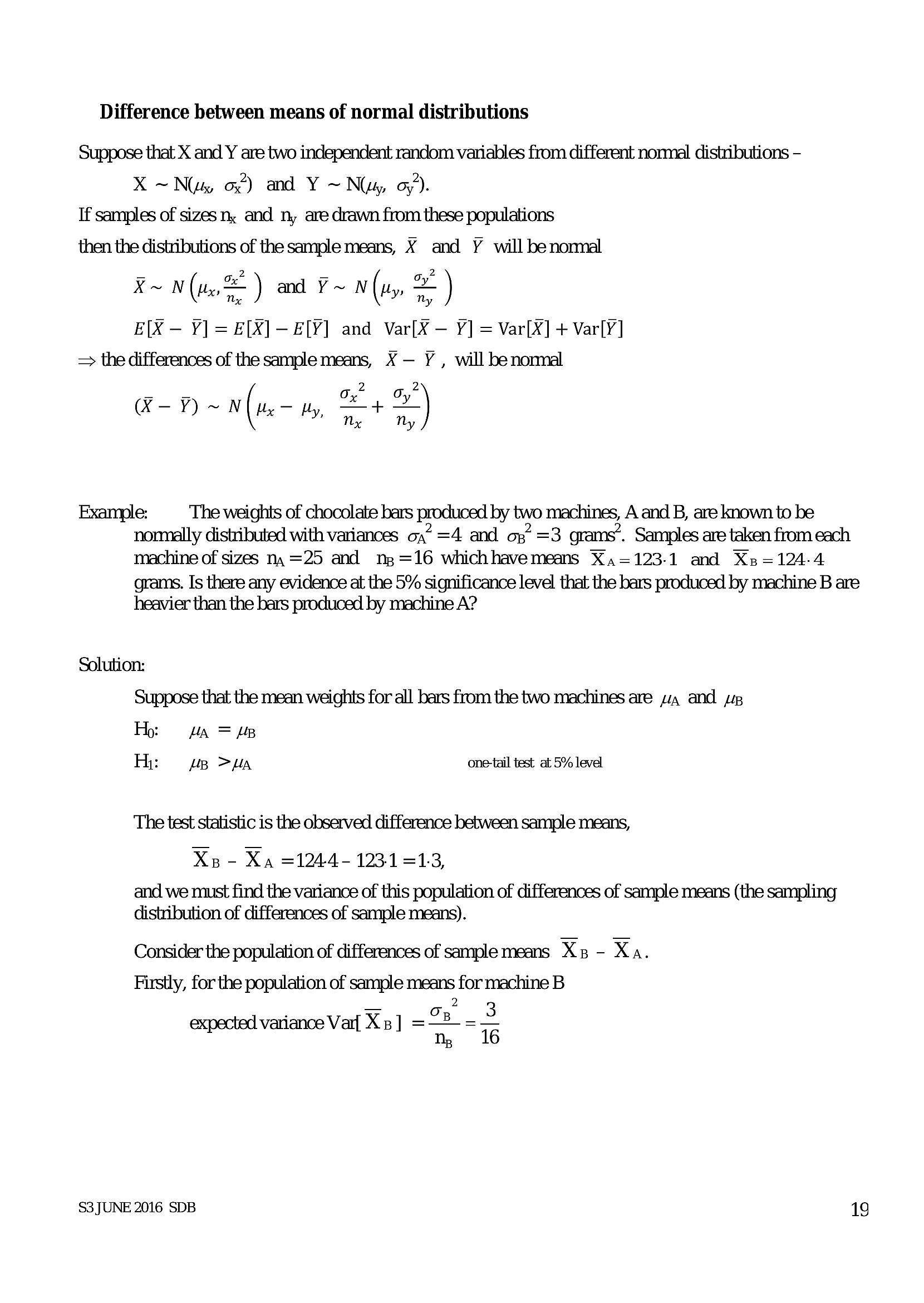
Difference between means of normal distributions

Suppose that X and Y are two independent random variables from different normal distributions -
X~ N(x o¢) and Y ~ Ny, oy).

If samples of sizes n, and ny are drawn from these populations

then the distributions of the sample means, X and Y will benormal

_ Ox? _ oy?

F~N (iS) and P~ NW (uy & )

E[X — Y] = E[X]-—E[Y] and Var[X — Y] = Var[X] + Var[Y]
=> the differences of the sample means, X — Y , will benonmal

(®-Y~N On,
Me Wy, ote

Example: The weights of chocolate bars produced by two machines, A and B, are known to be
nonmally distributed with variances on” =4 and o;” =3 grams’. Samples are taken from each
machine of sizes ny =25 and ng =16 whichhavemeans X,=123-1 and Xp=124-4
grams. Is there any evidence at the 5% significance level that the bars produced by machine B are
heavier than the bars produced by machine A?

Solution:
Suppose that the mean weights for all bars from the two machines are wa and pup
Ho: HA = 4B
Hi: up >a one-tail test at 5% level

The test statistic is the observed difference between sample means,

Xs - Xa =1244- 1231 =1:3,
and we must find the variance of this population of differences of sample means (the sampling
distribution of differences of sample means).
Consider the population of differences of sample means Xp - Xa.
Firstly, for the population of sample means for machine B
2
on 3

expected variance Var{ Xz ] =—=
n, 16

S3JUNE 2016 SDB 19

---

Page 22

Extracted Text

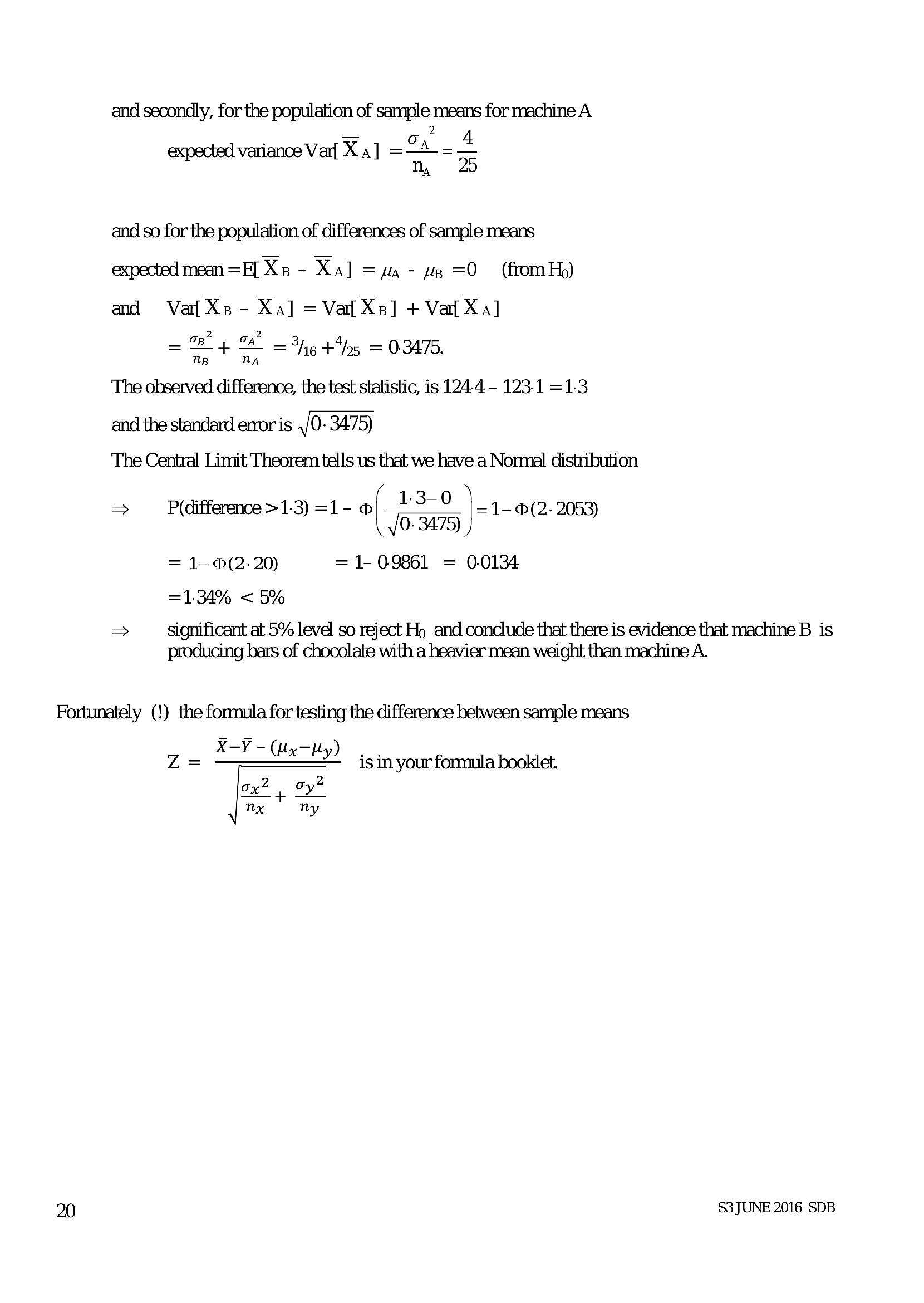
and secondly, for the population of sample means for machine A _ 2 expected variance Varf Xa] =24 = 4 Mm 25

and so for the population of differences of sample means
expected mean =E[ Xz - Xa] =a - wp =O (from Hy)
and Va Xe - Xa] =Vat Xs] + Vat Xa]

= oe oa 3h +405 = 03475.

np ny

The observed difference, the test statistic, is 124-4 - 123.1 =1.3
and the standard enoris ,/0- 3475)
The Central Limit Theorem tells us that we have a Nomnal distribution

. 1-3-0
> P(difference >1.3) =1- © =1-(2- 2053)
' a) (22053)
= 1- (2-20) = 1- 09861 = 0.0134

=134% < 5%

> significant at 5% level so reject Ho and conclude that there is evidence that machine B is
producing bars of chocolate with a heavier mean weight than machine A.

Fortunately (!) the formula for testing the difference between sample means

X-Y-(uy-Hy)
Z= AW¥ =x by) is in your formula booklet.
ox? | oy?
nx ny

20 S3JUNE 2016 SDB

---

Page 23

Extracted Text

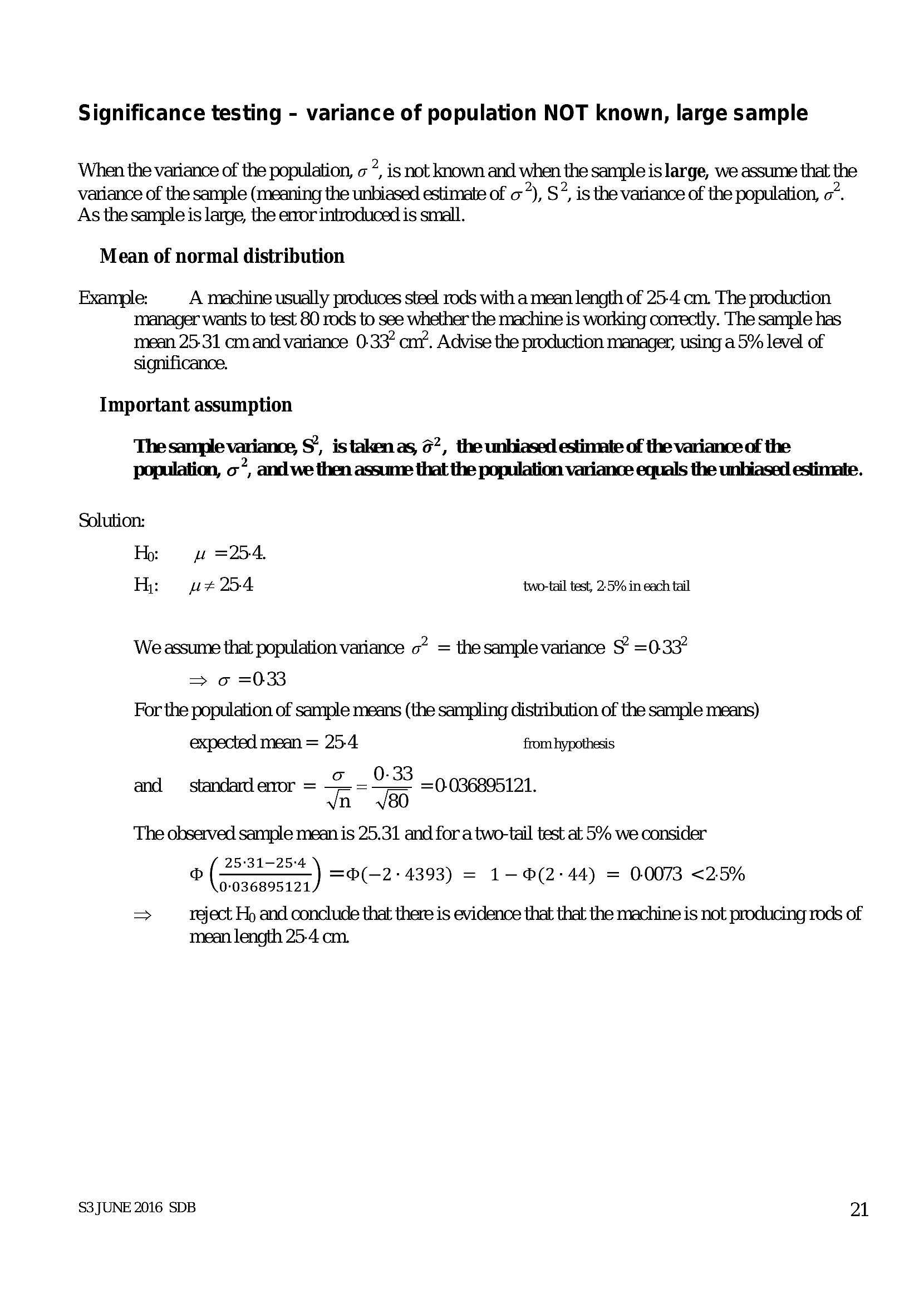
Significance testing - variance of population NOT known, large sample

When the variance of the population, « 7, is not known and when the sample is large, we assume that the
variance of the sample (meaning the unbiased estimate of o), S?, is the variance of the population, 0”.
As the sample is large, the eror introduced is small.

Mean of normal distribution

Example: A machine usually produces steel rods with a mean length of 25-4 cm. The production
manager wants to test 80 rods to see whether the machine is working correctly. The sample has
mean 25-31 cmand variance 0.33" cm’. Advise the production manager, using a 5% level of
significance.

Important assumption

The sample variance, S, istakenas, 62, the unhiased estimate of the variance of the
population, o?, and.we then assume that the population variance equals the unbiased estimate.

Solution:
Ho: “we =25-4.
H: w#254 two-tail test, 25% in each tail

We assume that population variance o” = the sample variance S’ =0-33?
> 0 =0:33
For the population of sample means (the sampling distribution of the sample means)
expected mean = 25-4 from hypothesis
o 0-33
and standard enor = Tn 80
The observed sample mean is 25.31 and for a two-tail test at 5% we consider
( 25:31-25:4
0-036895121
> reject Ho and conclude that there is evidence that that the machine is not producing rods of
mean length 25-4 cm.

=0-036895121.

) =@(-2 4393) = 1-(2:44) = 00073 <25%

S3JUNE 2016 SDB 21

---

Page 24

Extracted Text

Difference between means

Example:
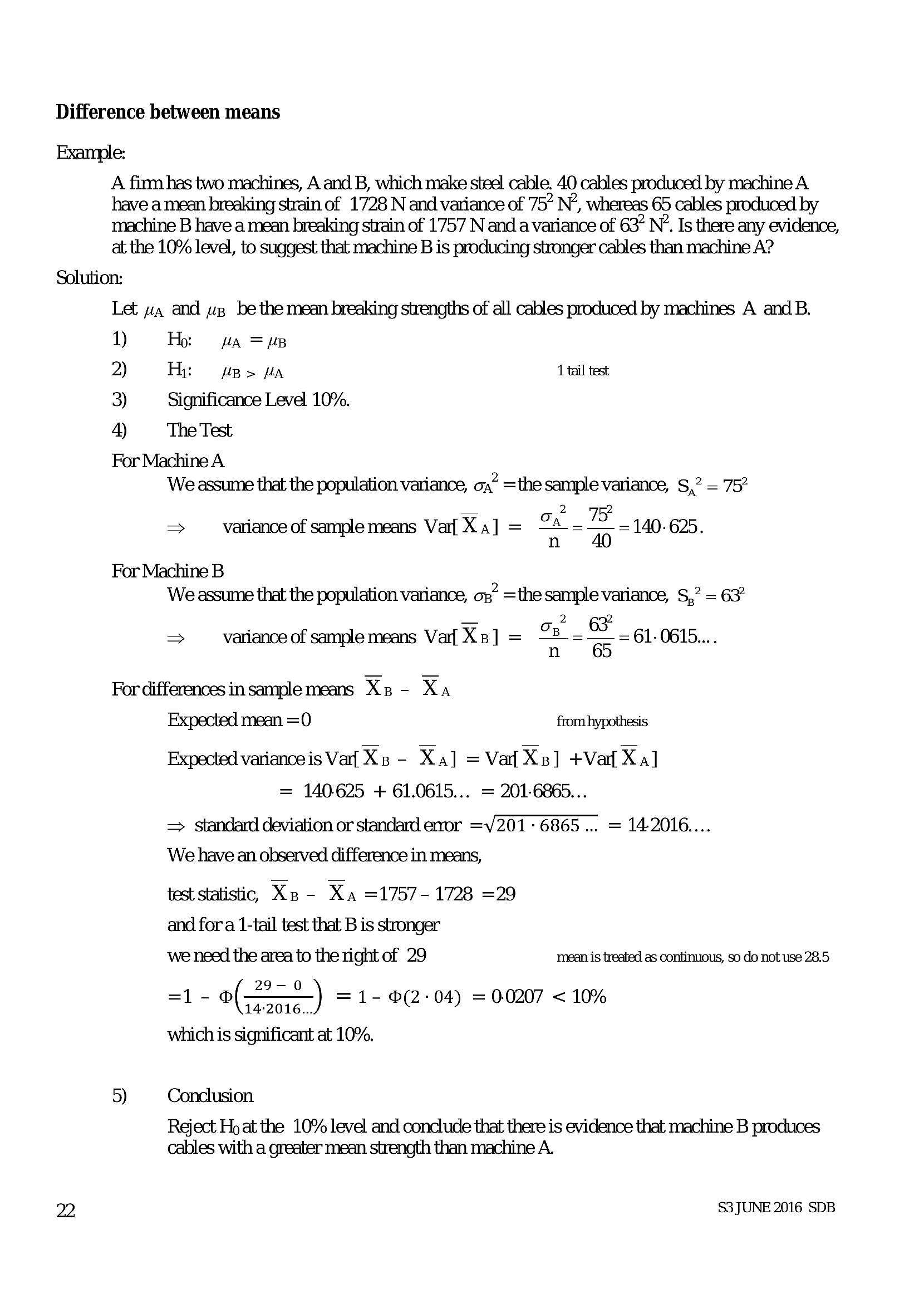
A firm has two machines, A and B, which make steel cable. 40 cables produced by machine A
have a mean breaking strain of 1728 N and variance of 75 N’, whereas 65 cables produced by
machine B have a mean breaking strain of 1757 N and a variance of 63 N*. Is there any evidence,
at the 10% level, to suggest that machine B is producing stronger cables than machine A?

Solution:
Let wa and zp be the mean breaking strengths of all cables produced by machines A and B.
1) Ho: wa =u

2 Hi vps wa 1 tail test
3) Significance Level 10%.
4) The Test
For Machine A
We assume that the population variance, o,” =the sample variance, S,? = 75°
— 2 2,
=> variance of sample means Var Xa] = Sa. 7 = 140-625.
For Machine B
We assume that the population variance, o;” =the sample variance, S,” = 63"

— 2
=> variance of sample means Var Xs] = ow 61-0616...
For differences in sample means Xp- Xa
Expected mean =0 from hypothesis
Expected variance is Varf Xn - Xa] =Vaf Xe] +Varl Xa]
= 140625 + 61.0615... = 201-6865...
=> standard deviation or standard exor =V 201-6865... = 14-2016....
We have an observed difference in means,

test statistic, Xp - Xa =1757- 1728 =29

and for a 1-tail test that B is stronger

we need the area to the right of 29 mean is treated as continuous, so do not use 28.5
29-0

=1- o(—) = 1- (2-04) = 0.0207 < 10%

which is significant at 10%.

5) Conclusion.

Reject Ho at the 10% level and conclude that there is evidence that machine B produces
cables with a greater mean strength than machine A.

oa) S3JUNE 2016 SDB

---

Page 25

Extracted Text

5 Goodness of fit, ” test

General points

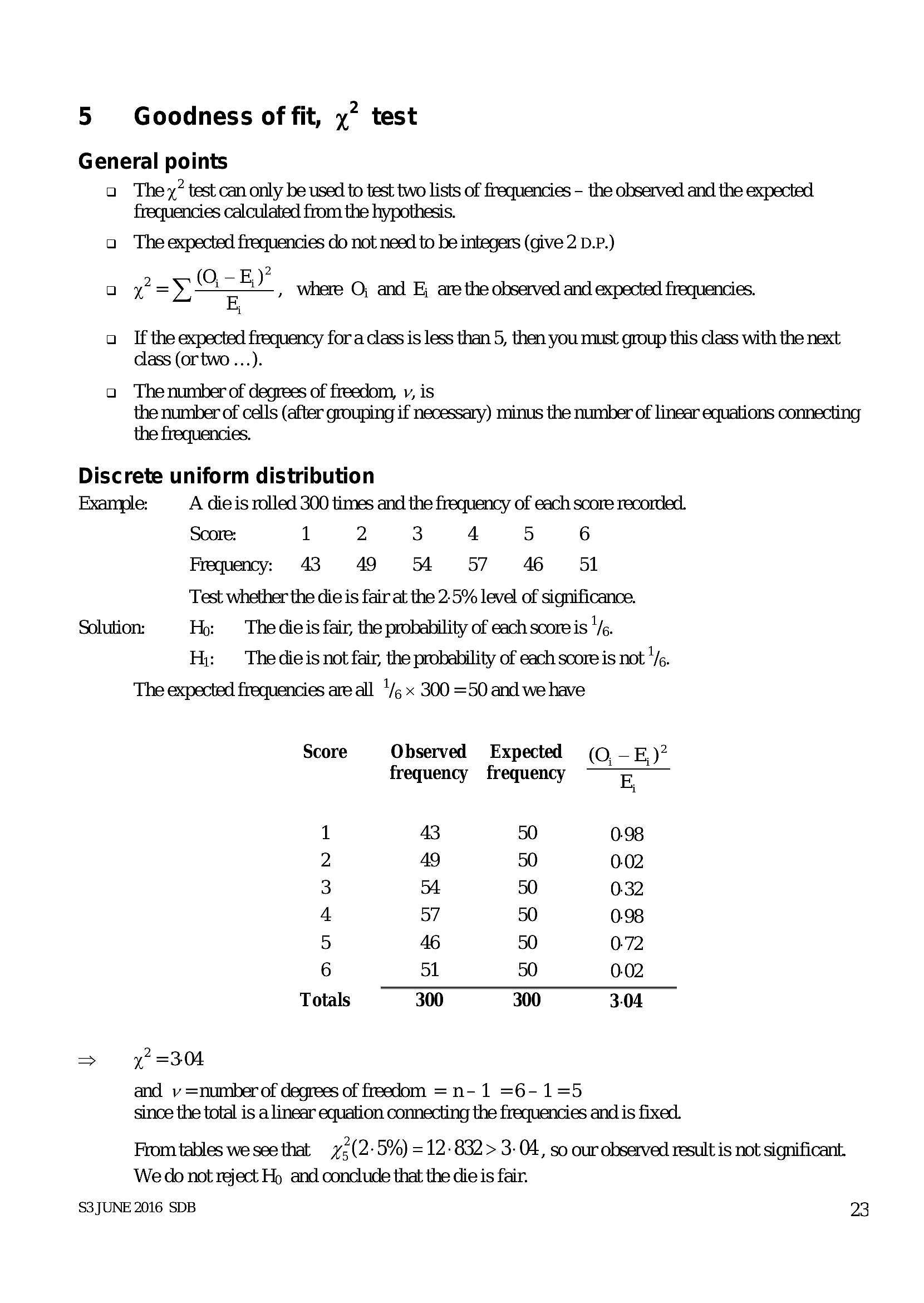
a The” test can only be used to test two lists of frequencies - the observed and the expected
frequencies calculated from the hypothesis.

a The expected frequencies do not need to be integers (give 2 D.P.)
2
a pay. where O; and E, are the observed and expected frequencies.

a If the expected frequency for a class is less than 5, then you must group this class with the next
class (or two ...).

a The number of degrees of freedom, v, is
the number of cells (after grouping if necessary) minus the number of linear equations connecting
the frequencies.

Discrete uniform distribution
Example: A dieis rolled 300 times and the frequency of each score recorded.

Score: 1 2 3 4 5 6
Frequency: 43 49 54 57 46 51
Test whether the die is fair at the 2.5% level of significance.
Solution: Ho: The dieis fair, the probability of each scoreis Y%.
H;: The dieis not fair, the probehility of each score is not ¥.
The expected frequencies are all 1/5 x 300 =50 and we have

Score Observed Expected (O,- 5)’
frequency frequency Ez

1 43 50 0.98
2 49 50 0.02
3 34 50 0.32
4 57 50 0.98
5 46 50 0-72
6 ol 50 0.02
Totals 300 300 3-04

> (=30
and v =number of degrees of freedom = n- 1 =6-1=5
since the total is a linear equation connecting the frequencies and is fixed.
From tables we see that 72(2-5%) = 12-832 > 3-04, so our observed result is not significant
We do not reject Hp and conclude that the die is fair.
S3JUNE 2016 SDB 23

---

Page 26

Extracted Text

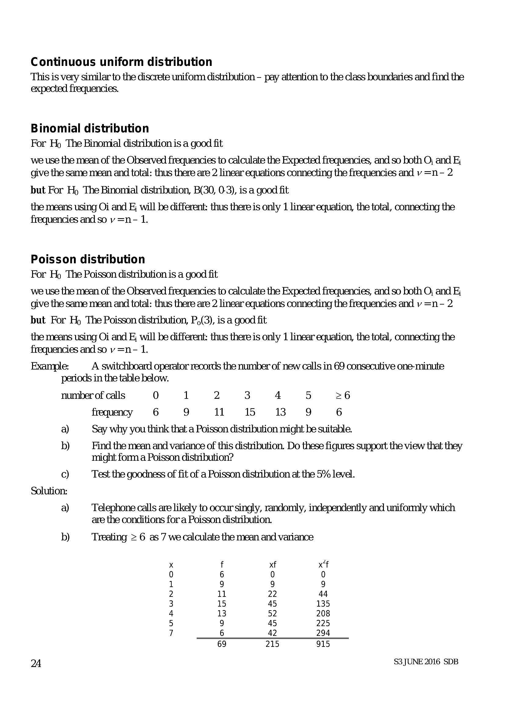
Continuous uniform distribution This is very similar to the discrete uniform distribution - pay attention to the class boundaries and find the expected frequencies.

Binomial distribution
For Hp The Binomial distribution is a good fit

we use the mean of the Observed frequencies to calculate the Expected frequencies, and so both O; and Ej
give the same mean and total: thus there are 2 linear equations connecting the frequencies and v =n- 2

but For Hy The Binomial distribution, B(30, 0-3), is a good fit
the means using Oi and F; will be different: thus there is only 1 linear equation, the total, connecting the
frequencies andso v =n - 1.

Poisson distribution
For Hp The Poisson distribution is a good fit

we use the mean of the Observed frequencies to calculate the Expected frequencies, and so both O; and Ej
give the same mean and total: thus there are 2 linear equations connecting the frequencies and v =n - 2
but For Hp The Poisson distribution, P,(3), is a good fit

the means using Oi and F; will be different: thus there is only 1 linear equation, the total, connecting the
frequencies and so v =n - 1.

Example: A switchboard operator records the number of new calls in 69 consecutive one-minute
periods in the table below.

number of calls 0 1 2 3 4 Fs) >6
frequency 6 9 11 15 13 9 6
a) Say why you think that a Poisson distribution might be suitable.

b) Find the mean and variance of this distribution. Do these figures support the view that they
might forma Poisson distribution?

c) Test the goodness of fit of a Poisson distribution at the 5% level.
Solution:

a) Telephone calls are likely to occur singly, randomly, independently and uniformly which
are the conditions for a Poisson distribution.

b) Treating > 6 as '7 we calculate the mean and variance

x f xf x‘f
0 6 0 0
1 9 9 9
2 11 22 44
3 15 45 135
4 13 52 208
5 9 45 225
7 6 42 294
69 215 915

2A S3 JUNE 2016 SDB

---

Page 27

Extracted Text

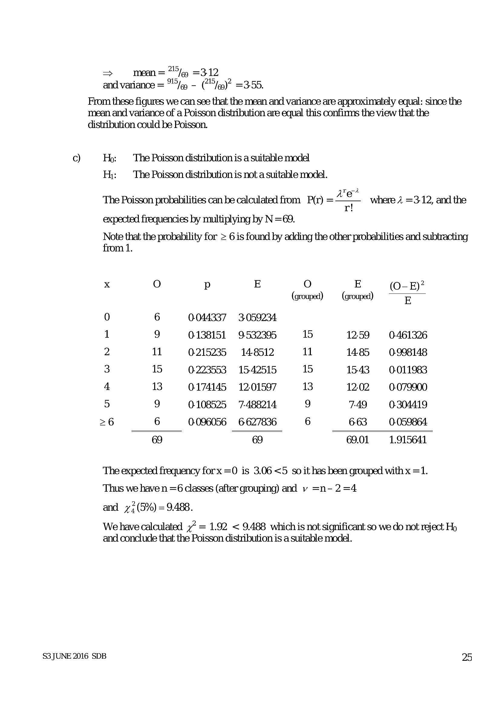
=> mean= "fg =3.12 and variance = fg - (7"5/eg)? =3.55. From these figures we can see that the mean and variance are approximately equal: since the

mean and variance of a Poisson distribution are equal this confirms the view that the
distribution could be Poisson.

c) Hp: — The Poisson distribution is a suitable model
H;: The Poisson distribution is not a suitable model.
A r e*

n where 2 =3-12, and the

The Poisson probabilities can be calculated from P(r) =

expected frequencies by multiplying by N =69.
Note that the probability for > 6 is found by adding the other probabilities and subtracting

from 1.
x O p E O E (O-E)?
(grouped) (grouped) E

0 6 0.044337 3059234

1 9 0138151 9532395 15 1259 0461326

2 11 0215235 14-8512 11 148 0998148

3 15 0-223553 1542515 15 1543 0.011983

4 13 0.174145 1201597 13 1202 0.079900

5 0108525 =7-488214 9 7-49 0.304419

>6 6 0.096056 6627836 6 663 0.059864
69 69 69.01 1.915641

The expected frequency forx =0 is 3.06 <5 so it has been grouped with x =1.
Thus we have n =6 classes (after grouping) and v =n- 2 =4
and 72(5%) = 9.488.

We have calculated 7” = 1.92 < 9.488 whichis not significant so we do not reject Hp
and conclude that the Poisson distribution is a suitable model.

S3JUNE 2016 SDB 25

---

Page 28

Extracted Text

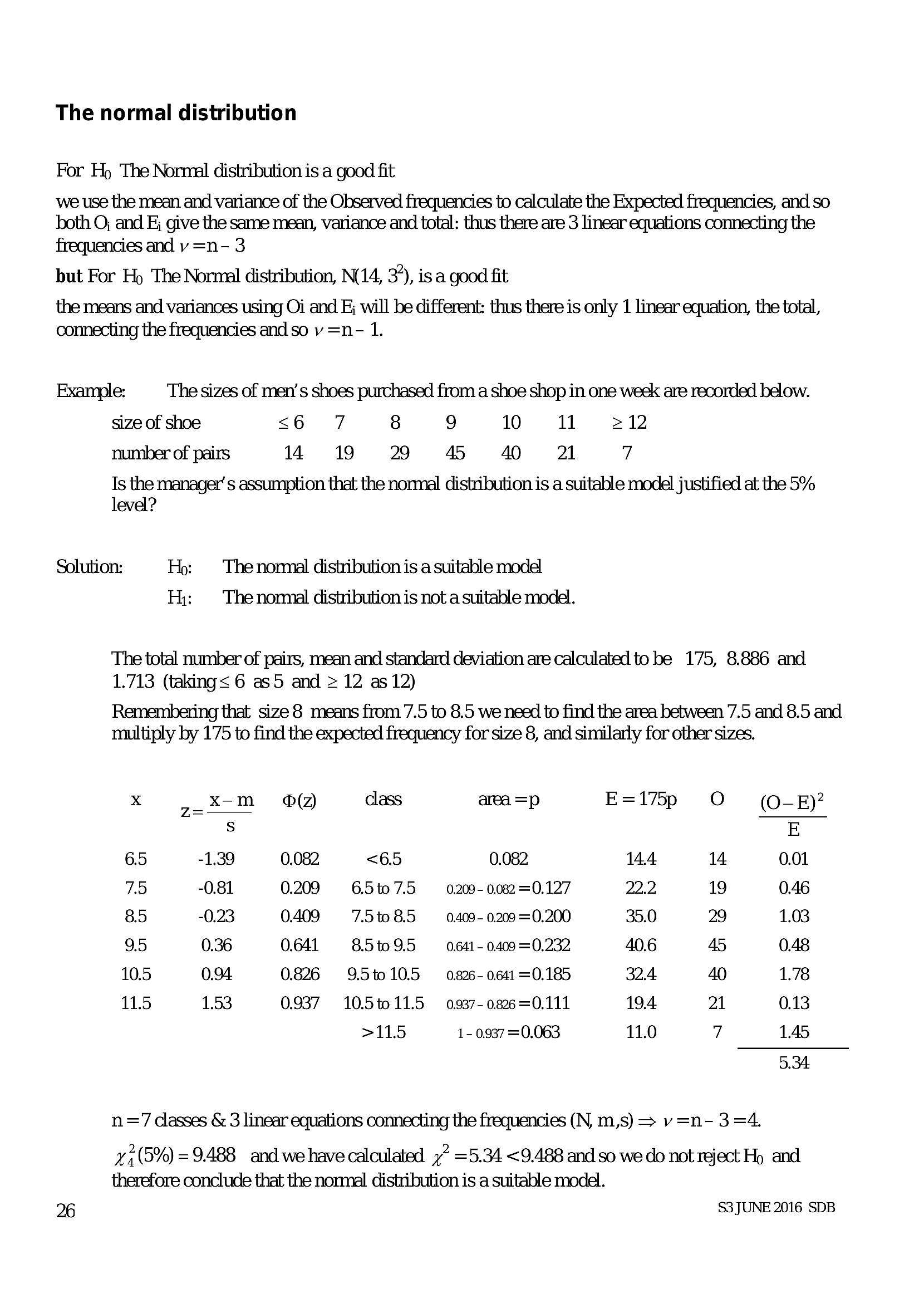
The normal distribution

For Hp The Nornal distribution is a good fit

we use the mean and variance of the Observed frequencies to calculate the Expected frequencies, and so
both O; and E; give the same mean, variance and total: thus there are 3 linear equations connecting the
frequencies and vy =n- 3

but For Hy The Normal distribution, N14, 3%, isa good fit

the means and variances using Oi and F; will be different: thus there is only 1 linear equation, the total,
connecting the frequencies and so v =n- 1.

Example: The sizes of men’s shoes purchased from a shoe shop in one week are recorded below.
size of shoe <6 7 8 9 10 11 >12
number of pairs 4 19 29 4 4 21 7

Is the manager’ s assumption that the normal distribution is a suitable model justified at the 5%
level?

Solution: Hp: | The normal distribution is a suitable model
H;: Thenormal distribution is not a suitable model.

The total number of pairs, mean and standard deviation are calculated to be 175, 8.886 and
1.713 (taking< 6 as5 and > 12 as 12)

Remembering that size 8 means from 7.5 to 8.5 we need to find the area between 7.5 and 8.5 and
multiply by 175 to find the expected frequency for size 8, and similarly for other sizes.

x go Xom (2) Class area =p E=175p oO (O-E)?
s E

65 -1.39 0.082 <6.5 0.082 144 14 0.01
7.5 -0.81 0.209 6.5t0 7.5 — 0.209- 0.082 =0.127 22.2 19 0.46
85 -0.23 0.409 7.510 8.5 — 0.409- 0.209 =0.200 35.0 29 1.03
9.5 0.36 0.641 8.5t09.5 0641-0409 =0.232 40.6 45 0.48
10.5 0.94 0.826 9.5t010.5 0826-0641 =0.185 32.4 40 1.78
11.5 1.53 0.937 10.5t011.5 0937-0826=0.111 19.4 21 0.13
>115 1- 0937 =0.063 11.0 7 1.45

5.34

n=7 Classes & 3 linear equations connecting the frequencies (N, m,s) > v=n- 3 =4.

713,6%) = 9.488 and we have calculated 7” =5.34 <9.488 and so we do not reject Hy and
therefore conclude that the normal distribution is a suitable model.

26 S3JUNE 2016 SDB

---

Page 29

Extracted Text

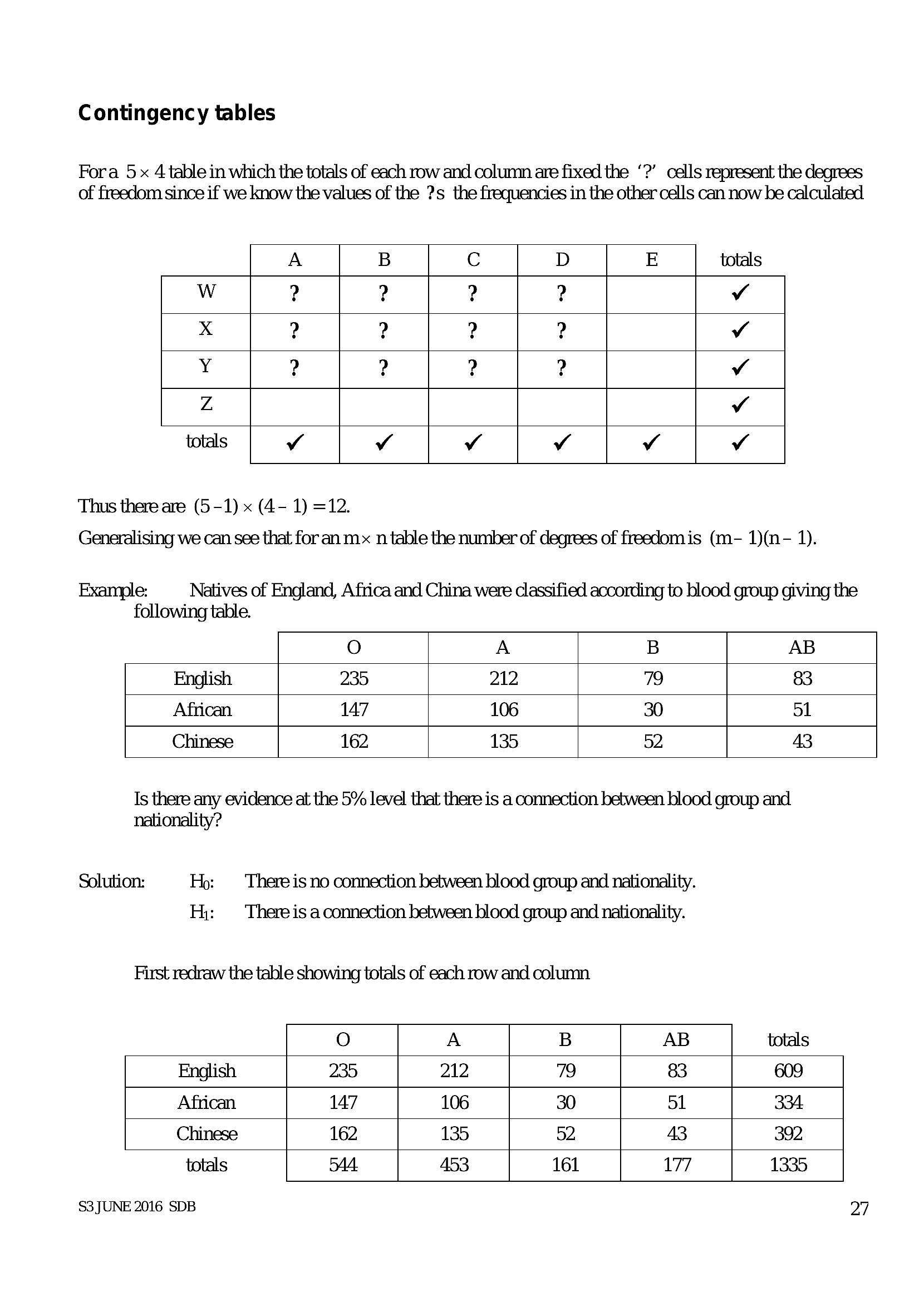
Contingency tables

Fora 5x 4 table in which the totals of each row and column are fixed the ‘?’ cells represent the degrees
of freedom since if we know the values of the ?s_ the frequencies in the other cells can now be calculated

A B Cc D E totals
w ? ? ? ? v
x ? ? ? ? v
Y ? ? ? ? v
Z v
totals | v v v v v

Thus there are (5-1) x (4- 1) =12.
Generalising we can see that for an mx n table the number of degrees of freedomis (m- 1)(n- 1).

Example: Natives of England, Africa and China were classified according to blood group giving the

following table.
O A B AB
English 235 212 79 83
African 147 106 30 Sl
Chinese 162 135 52 43

Is there any evidence at the 5% level that there is a connection between blood group and
nationality?

Solution: Hp: Thereis no connection between blood group and nationality.
H,;: There is aconnection between blood group and nationality.

First redraw the table showing totals of each row and column

O A B AB totals

English 235 212 79 83 609
African 147 106 30 Sl 334
Chinese 162 135 52 43 392
totals 44 453 161 177 1335

S3JUNE 2016 SDB 27

---

Page 30

Extracted Text

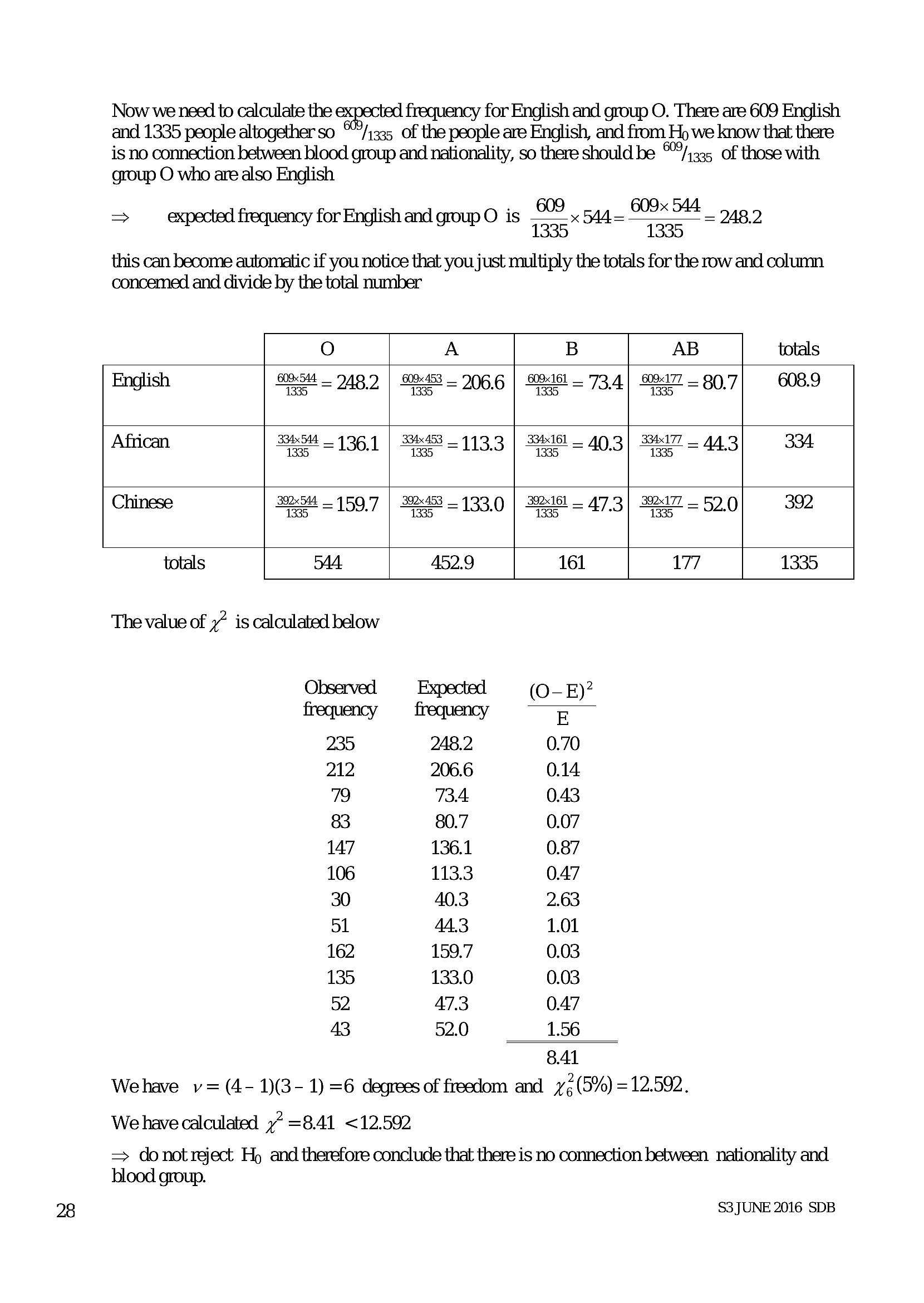
Now we need to calculate the frequency for English and group O. There are 609 English and 1335 people altogether so **/1335 of the people are English, and from Hp we know that there is no connection between blood group and nationality, so there should be ™/1335, of those with group O who are also English

609 609x 544
expected frequency for English and O is = =
> group" 18 7335 * 1335

this can become automatic if you notice that you just multiply the totals for the row and column
concemed and divide by the total number

248.2

O A B AB totals
English BSI _ 248. | SBs453 — 206,6 | 9245 - 73,4] SBA7 — 80,7} 608.9
African Sh _ 1361 | S453 113.3 ] Setst — 40.3] a7 _ 443] 334
Chinese a7-544 159.7 | X53 - 133.0 | S2do1- 47,3) S27 52.0) 392

totals 54 452.9 161 177 1335

The value of 7” is calculated below

Observed Expected (O-E)?
frequency frequency E

235 248.2 0.70
212 206.6 0.14
79 TBA 0.43

83 80.7 0.07

147 136.1 0.87
106 113.3 0.47
30 40.3 2.63

Sl 44.3 1.01

162 159.7 0.03
135 133.0 0.03
52 47.3 0.47

43 52.0 1.56
8.41

Wehave v= (4- 1)(3- 1) =6 degrees of freedom and 72(5%) =12.592.
We have calculated 77 =8.41 <12.592

=> donotreject Ho and therefore conclude that there is no connection between nationality and
blood group.
S3JUNE 2016 SDB

---

Page 31

Extracted Text

6 Regression and correlation Spearman’s rank correlation coefficient

Ranking and equal ranks

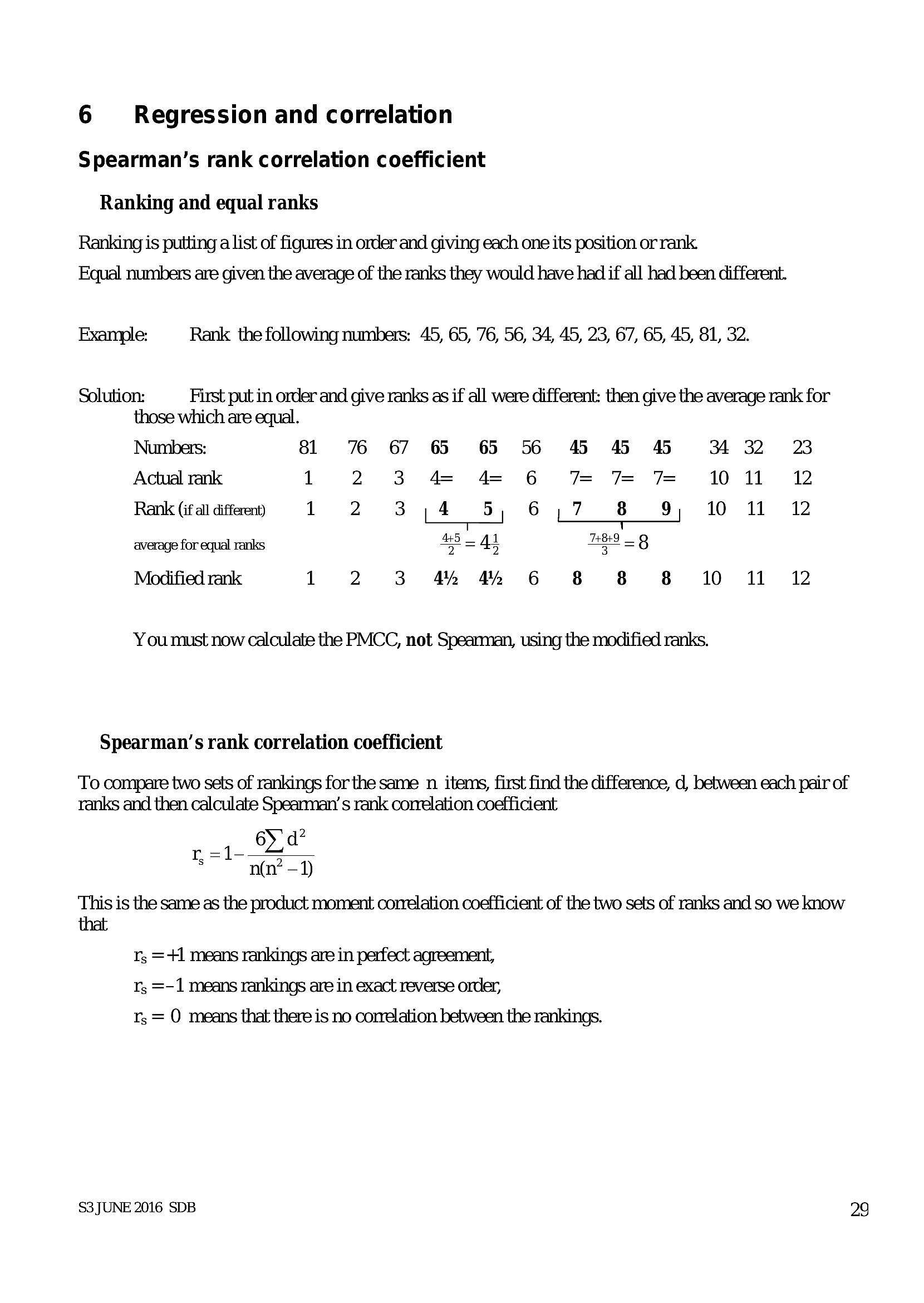
Ranking is putting a list of figures in order and giving each one its position or rank.
Equal numbers are given the average of the ranks they would have had if all had been different.

Example: Rank the following numbers: 45, 65, 76, 56, 34, 45, 23, 67, 65, 45, 81, 32.

Solution: First put in order and give ranks as if all were different: then give the average rank for

those which are equal.

Numbers: 81 7 67 6 6 56 6 4 4 4 32 2
Actual rank 1 2 3 4 4 6 7% 7 7 10 11 12
Rank (if all different) 1 2 3,4 =5 6,7 8 9 10 11 12
average for equal ranks 48-41 BE = 8

Modified rank 1 2 3 44 42 6 8 8 8 10 11 12

You must now calculate the PMCC, not Spearman, using the modified ranks.

Spearman’s rank correlation coefficient

To compare two sets of rankings forthe same n items, first find the difference, d, between each pair of
ranks and then calculate Spearman’ s rank correlation coefficient

6) d?
S =1- »
n(n‘ —1)

This is the same as the product moment correlation coefficient of the two sets of ranks and so we know
that

Ys =+1 means rankings are in perfect agreement,
Ys =-1 means rankings are in exact reverse order,
Ys = 0 means that there is no correlation between the rankings.

S3 JUNE 2016 SDB

29

---

Page 32

Extracted Text

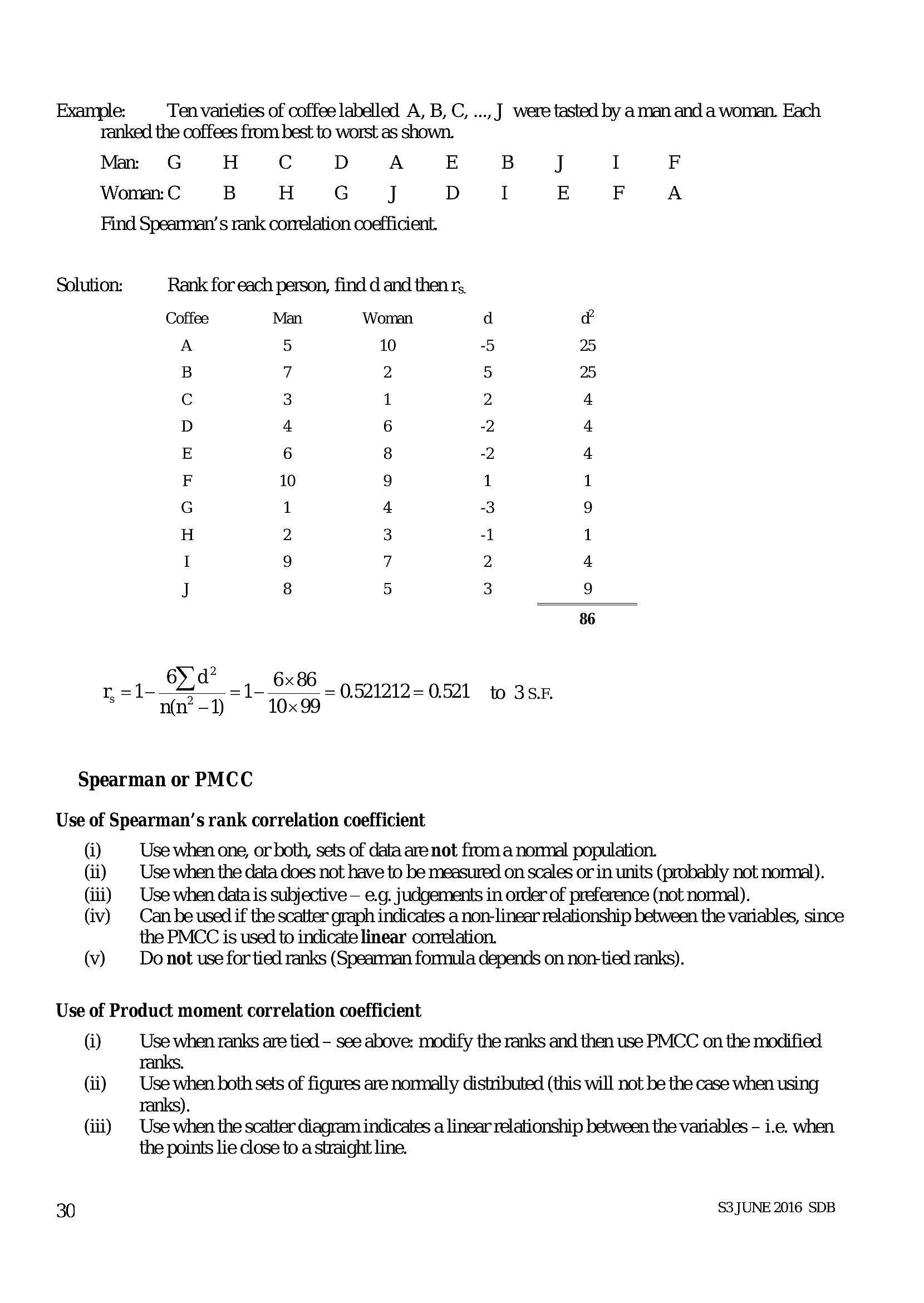
Example: Ten varieties of coffee labelled A, B, C, ..., J were tasted by aman and a woman. Each ranked the coffees from best to worst as shown.

Man: G H Cc D A E B J I F
Woman: C B H G J D I E F A
Find Speannan’s rank correlation coefficient.

Solution: Rank for each person, find d and then rs,
Coffee Man Woman

>
a
°
N
a

aA FwWN
WNAwWDEFENHONNO G 2
orF OP BB A

oSorertonmtmoodw
OONnNFRE
aun wh OD AMAEN

=<]
a

2
SDM" _ | 6x86

0.521212= 0.521 to 3sK
8 Tae) 10x99 SF

Spearman or PMCC

Use of Spearman’s rank correlation coefficient

(i) Use when one, or both, sets of data are not froma normal population.

(ii) Use when the data does not have to be measured on scales or in units (probably not nonnal).

(iii) | Use when data is subjective — e.g. judgements in order of preference (not normal).

(iv) | Can be used if the scatter graph indicates a non-linear relationship between the variables, since
the PMCC is used to indicate linear correlation.

(v) Do not use for tied ranks (Spearman formula depends on non-tied ranks).

Use of Product moment correlation coefficient
(i) Use when ranks are tied - see above: modify the ranks and then use PMCC on the modified

ranks.

(ii) Use when both sets of figures are normally distributed (this will not be the case when using
ranks).

(iii) | Use when the scatter diagram indicates a linear relationship between the variables - i.e. when
the points lie close to a straight line.

30 S3 JUNE 2016 SDB

---

Page 33

Extracted Text

Testing for zero correlation N.B. _ the tables give figures for a ONE-TAIL test

Product moment correlation coefficient

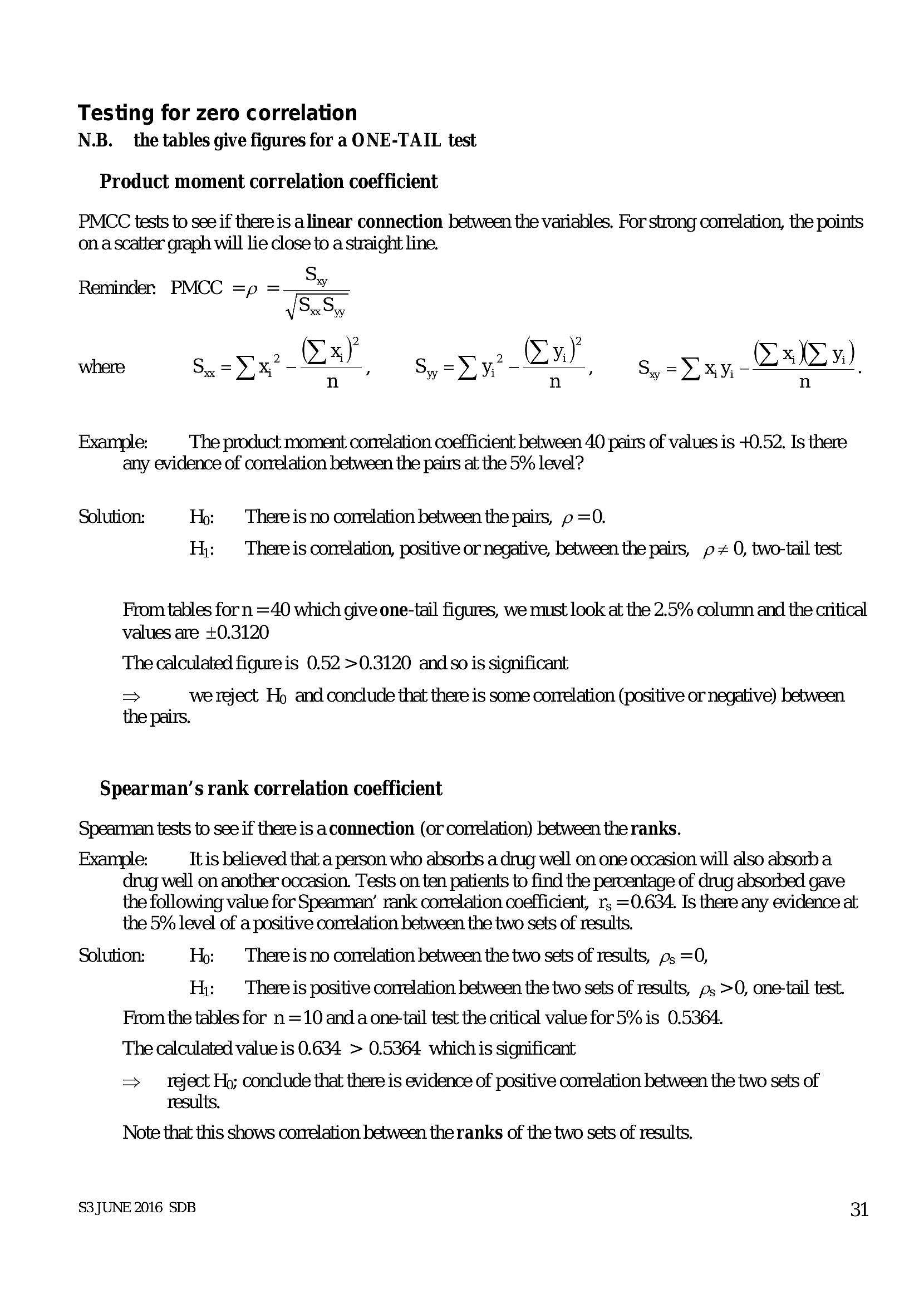
PMCC tests to see if there is a linear connection between the variables. For strong correlation, the points
on a scatter graph will lie close to a straight line.

S
Reminder PMCC =p =

x yy

S
2

ay 5.-Yy. Daal 5, <Dxy, (Xxoy)

where Sx =X ;

,

Example: The product moment correlation coefficient between 40 pairs of values is +0.52. Is there
any evidence of correlation between the pairs at the 5% level?

Solution: Hp: ‘There is no conelation between the pairs, p =0.
H,: Thereis conelation, positive or negative, between the pairs, = 0, two-tail test

From tables forn =40 which give one-tail figures, we must look at the 2.5% column and the critical
values are +0.3120

The calculated figureis 0.52 >0.3120 and so is significant

> we reject Hp and conclude that there is some correlation (positive or negative) between
the pairs.

Spearman’s rank correlation coefficient

Spearman tests to see if there is a connection (or correlation) between the ranks.

Example: Itis believed that a person who absorbs a drug well on one occasion will also absorb a
drug well on another occasion. Tests on ten patients to find the percentage of drug absorbed gave
the following value for Spearman’ rank correlation coefficient, r; =0.634. Is there any evidence at
the 5% level of a positive correlation between the two sets of results.

Solution: Hp: There is no conelation between the two sets of results, ps =0,
H,: Thereis positive correlation between the two sets of results, ; >0, one-tail test.
From the tables for n =10 anda one-tail test the critical value for 5% is 0.5364.
The calculated value is 0.634 > 0.5364 which is significant

=> reject Hp; conclude that there is evidence of positive correlation between the two sets of
results.

Note that this shows correlation between the ranks of the two sets of results.

S3JUNE 2016 SDB 31

---

Page 34

Extracted Text

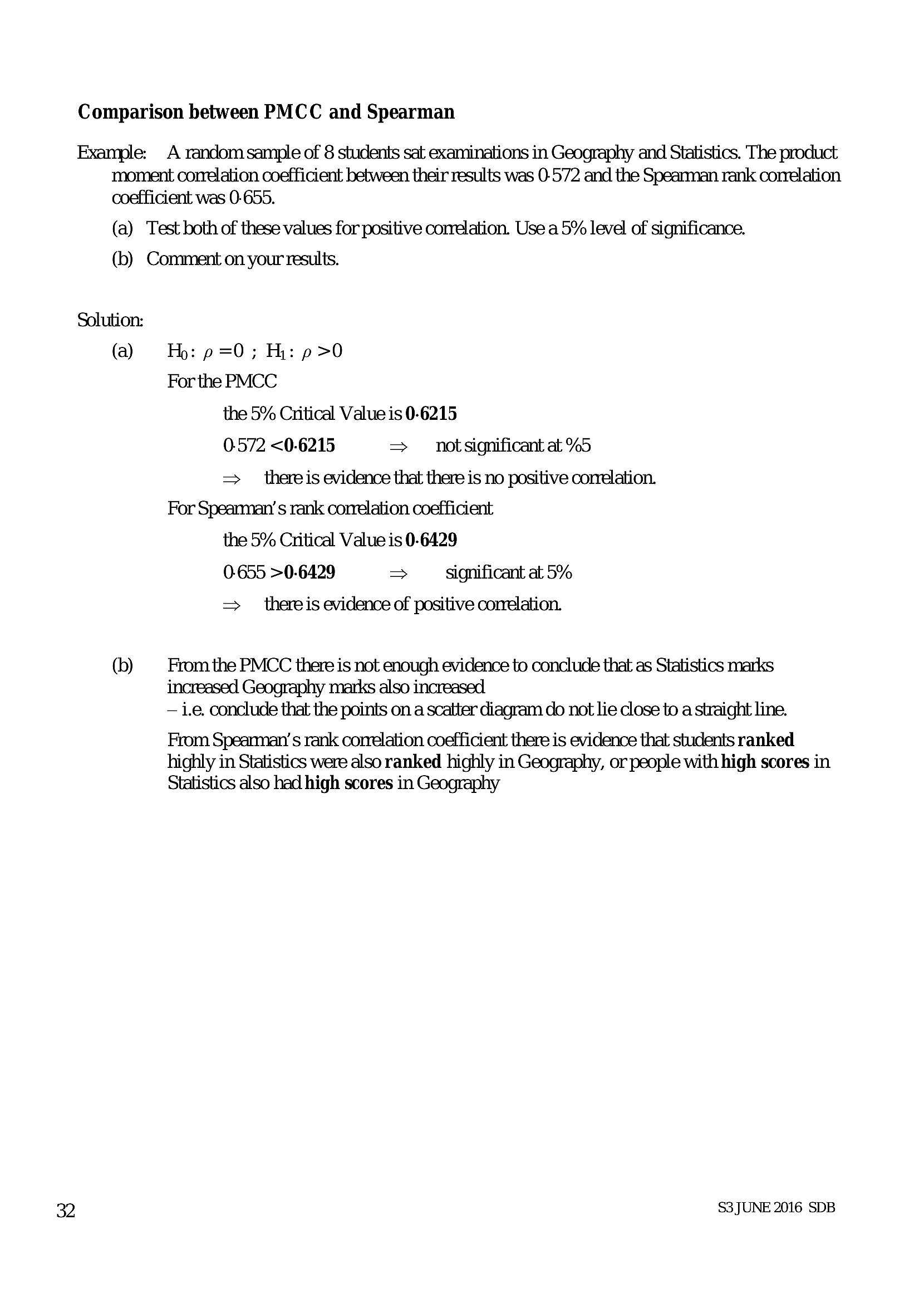
Comparison between PMCC and Spearman

Example: A random sample of 8 students sat examinations in Geography and Statistics. The product
moment correlation coefficient between their results was 0-572 and the Spearman rank correlation
coefficient was 0-655.

(a) Test both of these values for positive correlation. Use a 5% level of significance.
(b) Comment on your results.

Solution:
(a) Ho: p =0; Hi: p>0
For the PMCC
the 5% Critical Value is 0-6215

0.572 <0-6215 => notsignificant at %5

= _ thereis evidence that there is no positive correlation.
For Spearman’ s rank correlation coefficient

the 5% Critical Value is 0.6429

0-655 >0-6429 > significant at 5%

= _ thereis evidence of positive conelation.

(b) From the PMCC there is not enough evidence to conclude that as Statistics marks
increased Geography marks also increased.
— i.e. conclude that the points on a scatter diagram do not lie close to a straight line.
From Spearman ’s rank correlation coefficient there is evidence that students ranked
highly in Statistics were also ranked highly in Geography, or people with high scores in
Statistics also had high scores in Geography

ey) S3JUNE 2016 SDB

---

Page 35

Extracted Text

7 Appendix

Combining random variables

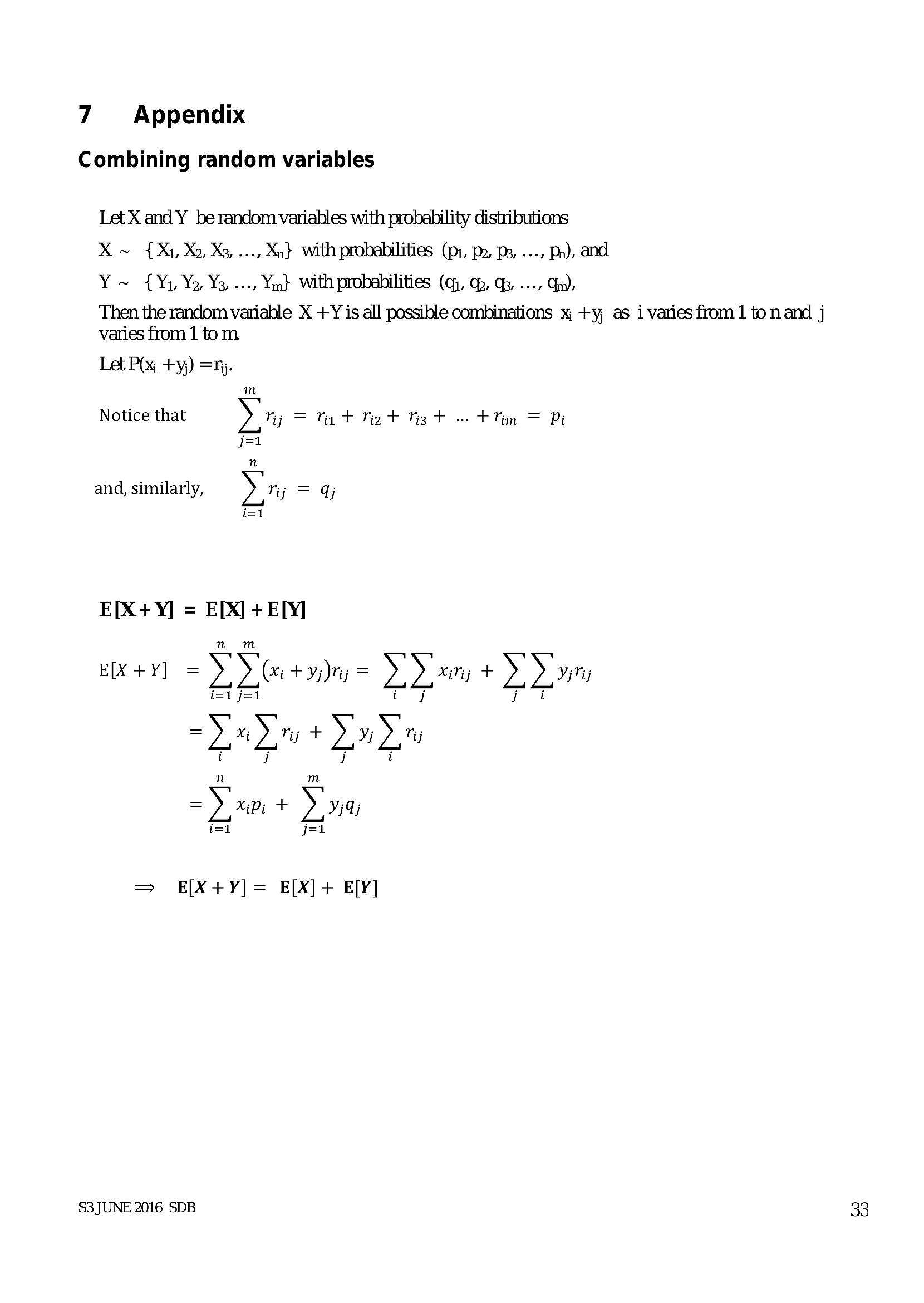
Let X and Y be random variables with probability distributions
X ~ {X, Xo, Xz, ..., Xn} with probabilities (pi, po, ps, ..., Pa), and
Y~ {Y1 Yo, Y3,..., Ym} with probabilities (qy, dp, q3, ..., Gm),

Then the random variable X +Y is all possible combinations % +yj as i varies from 1 to nand j
varies from 1 tom

Let PQ +yj) =Tj.
m
Notice that yy = N+ Tig + ig + we +lim = Yi
j=1
n

and, similarly, » ry = qj

i=1

E[X+Y] = E[X] + ETY]

(xi + y,)nj = dd* Nj + D2
j=l
Sn 4 Sod

J

m
XiDi + Ya

j=l

EIX+Y] =

Me:

I
RB

Ms Mw!

t

Il
RB

= E[X+¥]= E[X]+ EY]

S3 JUNE 2016 SDB

33

---

Page 36

Extracted Text

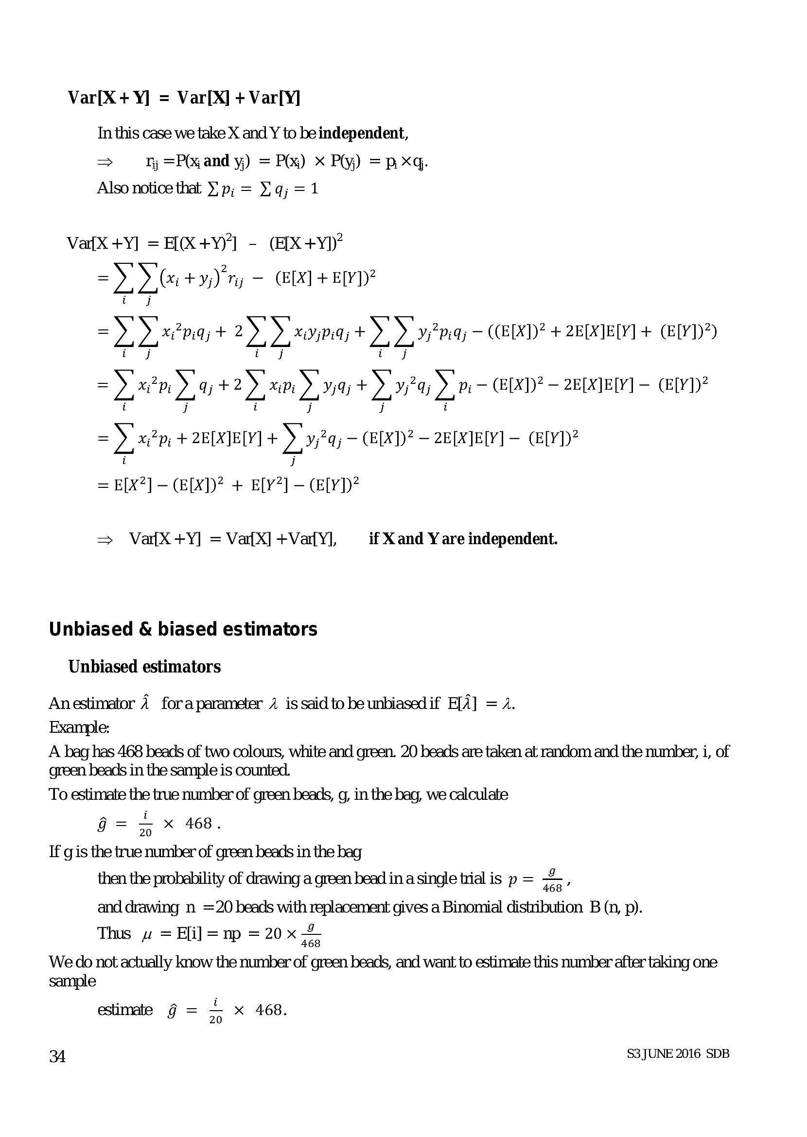
Var[X + Y] = Var[X] + Var[Y]

In this case we take X and Y to be independent,
=> 1 =Pand y) = PO) x Py) =p xq.
Also notice that }!p; = qj = 1

Va{X +¥] = E[(X+Y)"] - (FIX+yY))”
= xc +y;) Ty — ([X] + E[Y])?
ij

=) Yep; + 2) ) xiypiqy +>) yea) — (E[X)? + 2E[X]E[Y] + (E[Y])?)
i i if if

=) x2p. Ya +2) xm dy) + Dy?) > Pi— (ELD? — 2ELX1EY] - (E[Y])?
i j i j j i

=) xpi + 2ELXIED] +) 9424) — (EECD? - 2ELXTELY] - (BLY?
i i

= E[X?] — EX)? + Ely] - (ely)?

=> Vaf{X+Y] = VatX] +VaYl, if X and Y are independent.

Unbiased & biased estimators
Unbiased estimators

Anestimator 4 foraparameter 4 is said to be unbiasedif E[A] = A.

Example:

A bag has 468 beads of two colours, white and green. 20 beads are taken at random and the number, i, of
green beads in the sample is counted.

To estimate the true number of green beads, g, in the bag, we calculate

G= 5 x 468.
If gis the true number of green beads in the bag

then the probability of drawing a green bead in a single trial is p = <

and drawing n =20 beads with replacement gives a Binomial distribution B (n, p).

Thus w« = E[i]=np = 20x 4
We do not actually know the number of green beads, and want to estimate this number after taking one
sample

estimate g = = x 468.

34 S3 JUNE 2016 SDB

---

Page 37

Extracted Text

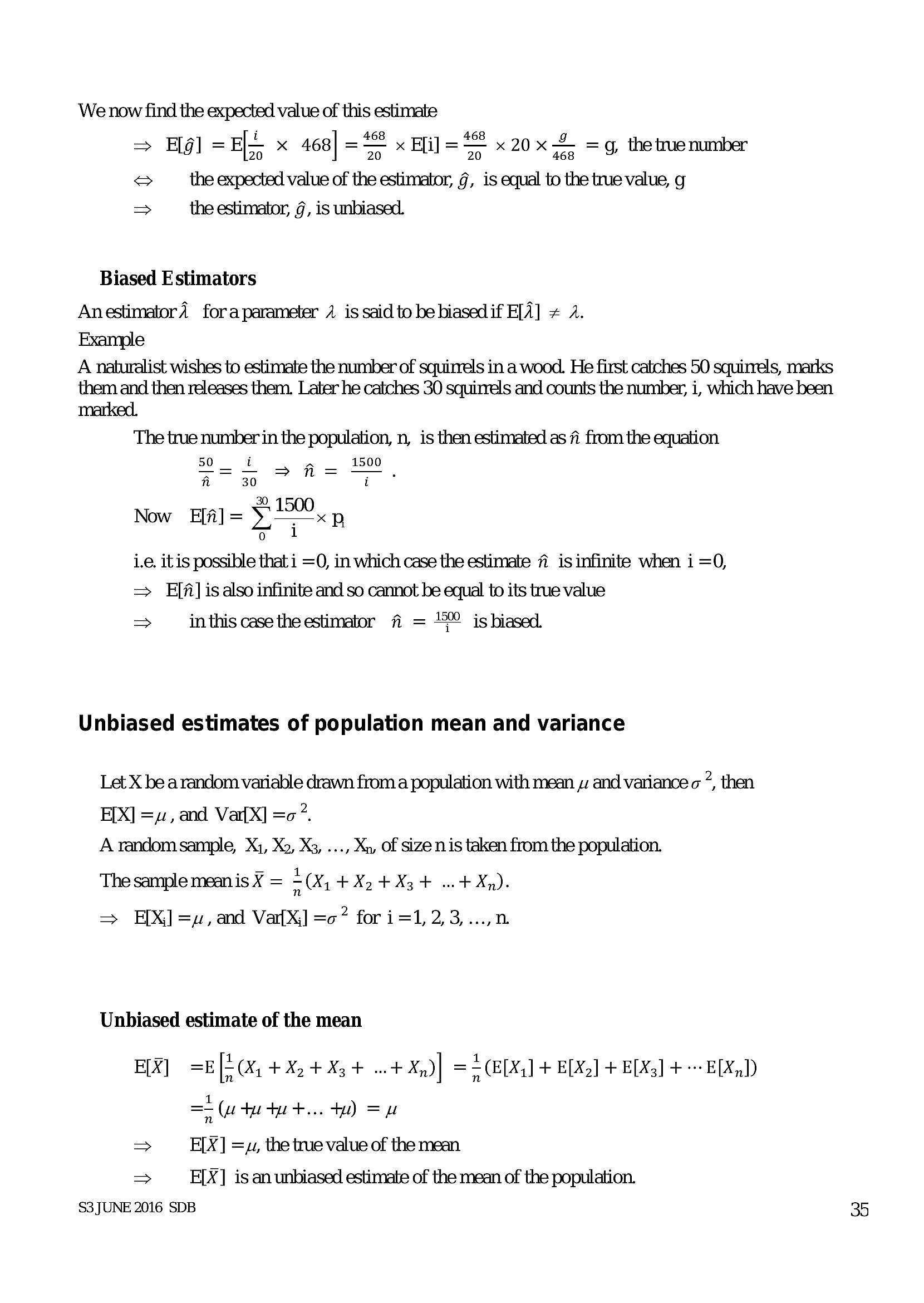
We now find the expected value of this estimate 68

> Hg = E- x 468] = <= x Eli] == x 20x =g, the true number

S the expected value of the estimator, g, is equal to the true value, g
> the estimator, g, is unbiased.

Biased Estimators
Anestimatord foraparameter / is said to bebiasedif E[A] # 4.

Example
A naturalist wishes to estimate the number of squirrels in a wood. He first catches 50 squirrels, marks
them and then releases them. Later he catches 30 squirrels and counts the number, i, which have been
marked.
The true number in the population, n, is then estimated as fi from the equation
50 i a 1500

= > n=
nr 30 i

30.
Now Ea] = 5°, 5
7 (i
ie. itis possible that i =O, in which case the estimate fi is infinite when i =0,
= Ef] is also infinite and so cannot be equal to its true value
=> inthiscasetheestimator A = 4 isbiased

i

Unbiased estimates of population mean and variance

Let X be a random variable drawn from a population with mean yw and variance o ’, then
E[X] =u, and Var[X] =o.

A random sample, Xi, X2, Xz, ..., Xn, of size n is taken from the population.

The sample mean is ¥ = =(X, +X. +X3+ ..+Xn).

=> EX) =, and Va{X] =c? for i=1,2,3,...,n

Unbiased estimate of the mean
FIX] =E[2(X%, +X, 4X34 «+ Xd] == CED] + ELXe] + BLX5] + EXD

=< (ututut... tw) =u
> E[X] =y, the true value of the mean
> E[X] is an unbiased estimate of the mean of the population.
S3 JUNE 2016 SDB

---

Page 38

Extracted Text

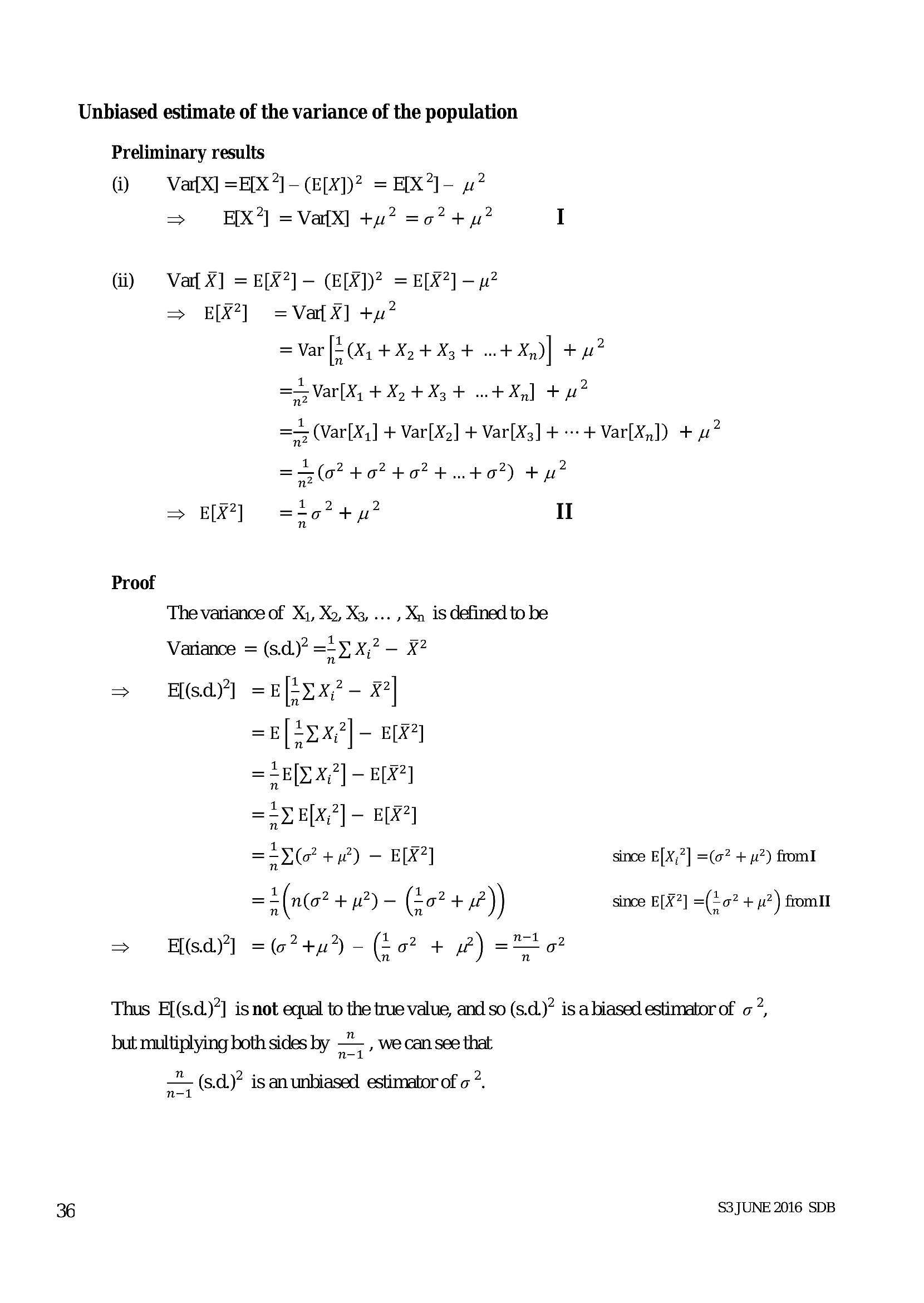
Unbiased estimate of the variance of the population Preliminary results @ = Va{X] =EIX?] - (E[X))? = EIX7]- wv? => EX?) =VaiX] tu? =07 +p? I

Gi) = Var X] = E[X?] — (E[X]))* = E[X?] — p?
=> EL] =Vat¥] tu?
= Var [= (X, +X, +X3 + + Xq)| + a?
=SVar[X, + Xp +X34+ + Xq] tu?
=5 (Var[X,] + Var[X,] + Var[X3] + «++ Var[X,,]) + we
=S(o? +02 +07 +..407) $y?

=> EL] =207 +p? II

Proof
The variance of X1, Xo, X3, ... , Xn is defined to be

Variance = (sd)? ==y, x,? — X?
= H(sd)} =E[;rx? - x|
=E[2Ex2| - ELX?]
= <b[D X;7] — E[X?]
=+Y E[X,?] - ELX?]
=23(o? +42) — BIR?) since E[X,?] =(0? + u2) from
=*(n(o? + 12) — (20? +4) since E[X?] =(20? + p?) from

=> H(sd)"] =? +p) - (20? + 2) =o?

Thus F[(s.d)”] is not equal to the true value, and so (s.d.)” is abiased estimator of o?,
but multiplying both sides by aa , we can see that
a (s.d.)* is an unbiased estimator of o .

S3 JUNE 2016 SDB

---

Page 39

Extracted Text

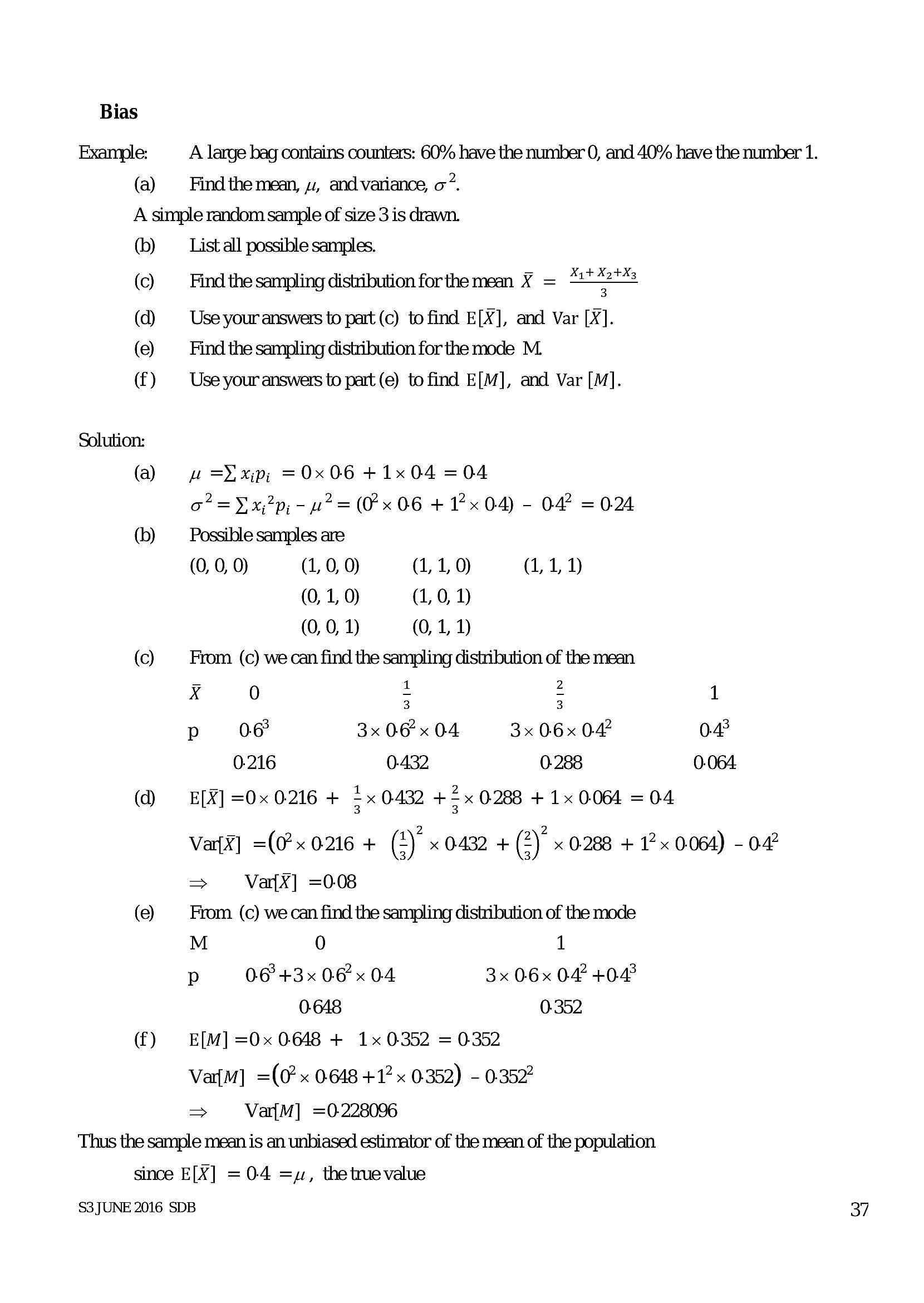
Bias

Example: A large bag contains counters: 60% have the number 0, and 40% have the number 1.
(a) Find the mean, yz, and variance, o?.
A simple random sample of size 3 is drawn.
(b) List all possible samples.
(Find the sampling distribution for the mean ¥ = “72%
(d) Use youranswers to part (c) to find E[X], and Var [X].
(2) Find the sampling distribution for the mode M.
(f) | Use your answers to part (e) to find E[M], and Var [M].

Solution:
(a wv =oxp, =0x064+1x04 =04
o*% =Yx2p; - w2 = (0x 06 + 12x 0-4) - 04 =0:24
(b) Possible samples are
(0, 0, 0) (1, 0, 0) (1, 1, 0) (1, 1, 1)
(0, 1, 0) (1, 0, 1)
(0, 0, 1) (0, 1, 1)
(co) From (c) we can find the sampling distribution of the mean

x 0 2 2 1
3 3
p oe 3x 06x 04 3x 06x 047 0.48
0.216 0-432 0-288 0.064

(@ — E[X] =0x 0216 + x 0432 += x 0-288 + 1x 0064 = 04

Vaz] =(x 0216 + (2) x 0432 + (2)° x 0288 + 1x 0064) - 04

> Var{X] =0-08
(e) From (c) we can find the sampling distribution of the mode

M 0 1
Pp 06°+3x 06x 04 3x 06x 04 +048
0-648 0-352

(f) E[M] =0x 0648 + 1x 0352 = 0352
VafM] =(0? x 0.648 +12 x 0352) - 0-352
> Va{M] =0228096
Thus the sample mean is an unbiased estimator of the mean of the population
since E[X] = 0-4 =, the truevalue

S3 JUNE 2016 SDB

---

Page 40

Extracted Text

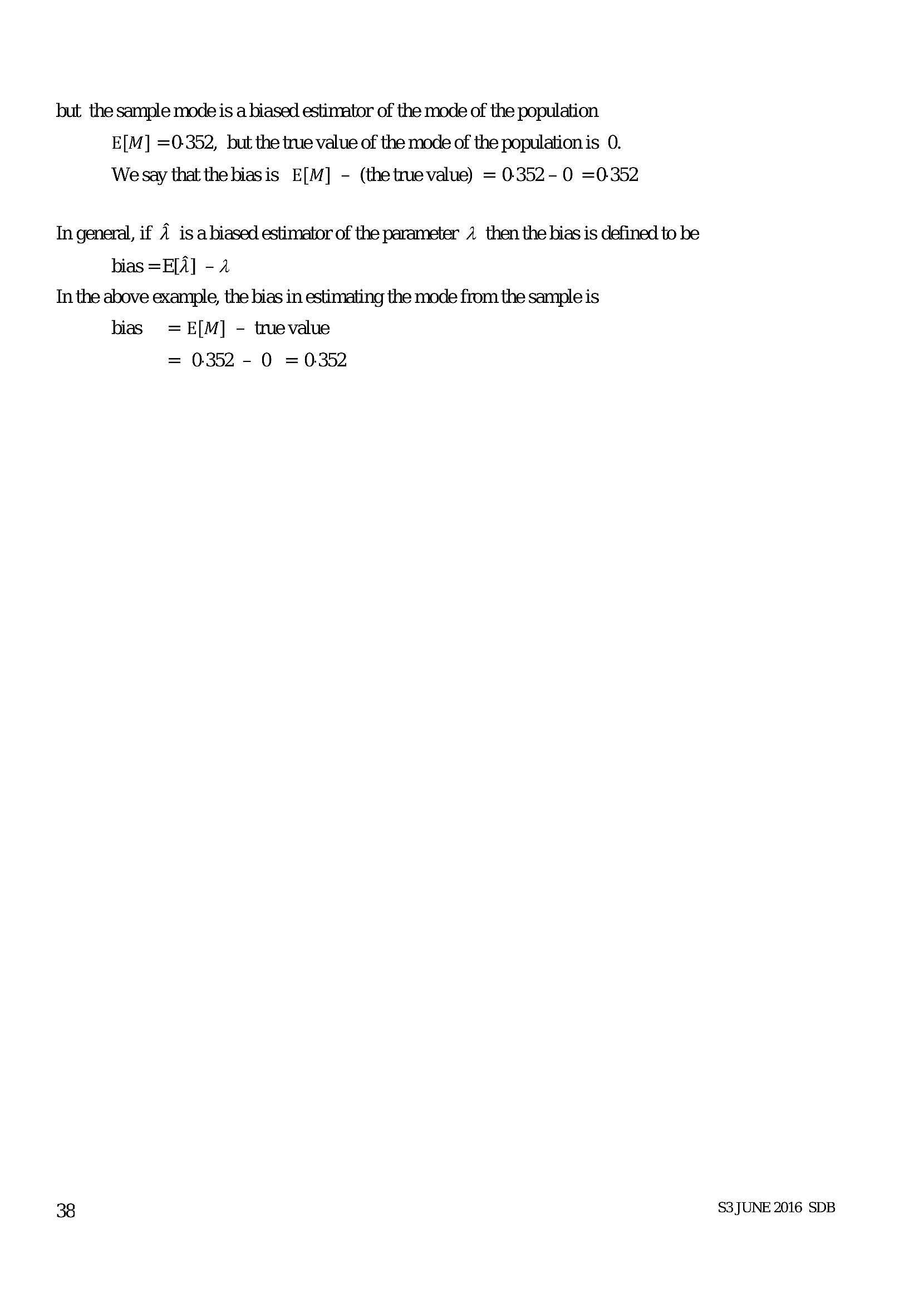
but the sample mode is a biased estimator of the mode of the population E[M] =0-352, but the true value of the mode of the population is 0. We say that thebiasis E[M] - (thetruevalue) = 0352-0 =0:352

In general, if 7 is abiased estimator of the parameter 4 then the bias is defined to be
bias =E[A] - 2
In the above example, the bias in estimating the mode from the sample is
bias =E[M] - tevalue
= 0352 - 0 =0.352

S3 JUNE 2016 SDB

---

Page 41

Extracted Text

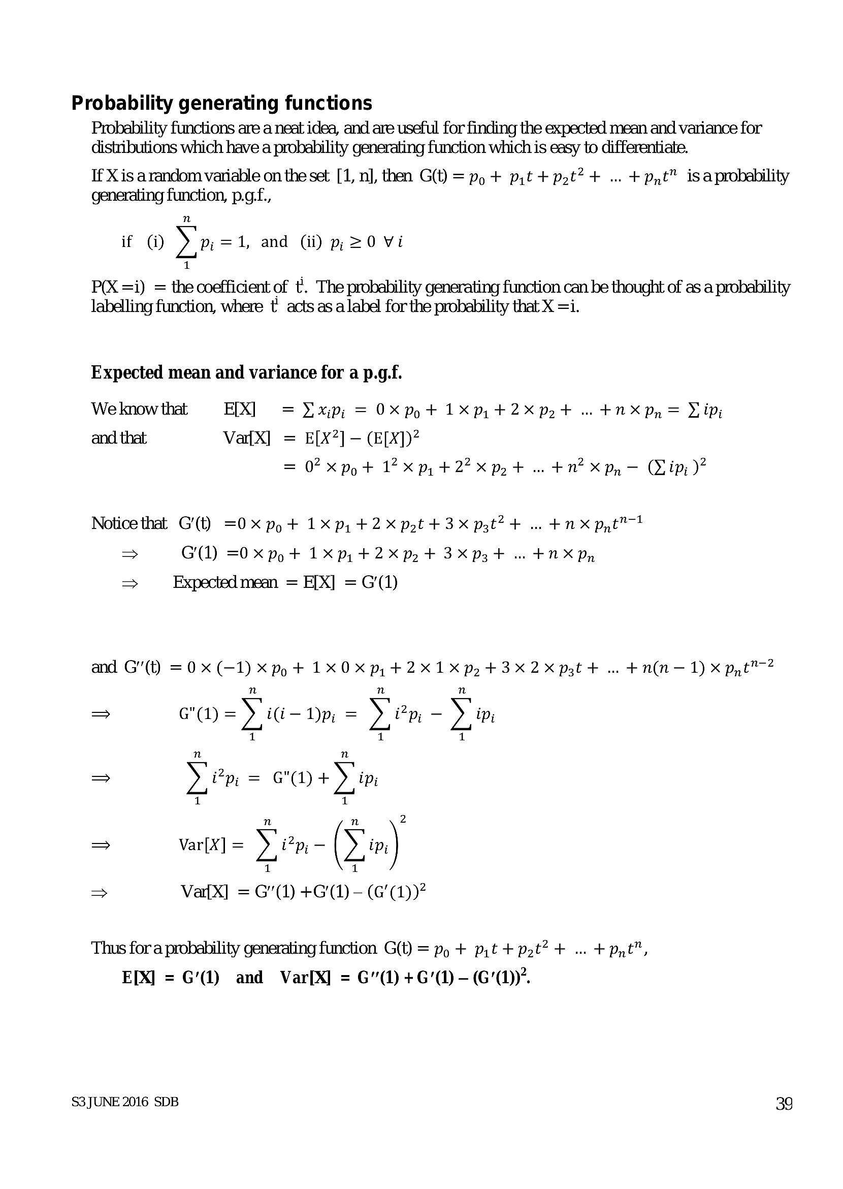
Probability generating functions Probability functions are a neat idea, and are useful for finding the expected mean and variance for distributions which have a probability generating function which is easy to differentiate. If Xis arandom variable on the set [1, n], then G(t) = pop + pyt + pt? + ... + pyt™ isaprobability generating function, p.g.f.,

n
if (i Yat and (ii) pj =0 Vi
1

P(X =i) = the coefficient of t!. The probability generating function can be thought of as a probability
labelling function, where t° acts as alabel for the probability that X =i.

Expected mean and variance for a p.g.f.
We know that EX] = Yxp; = Oxppt1xpyt+2xprt .. +nX py = Lip;
and that VatX] = E[X?] - (E[X])?

= 0? xpot 17x p, +227x pot... $n? xX p,— (Vip; )?

Notice that G’(t) =0x po + 1p, +2 pot +3 pst? + .. +n X ppt?
> G(1) =O x pop t+ 1X py t+2X pot 3Xpzgt .. #NX Dy
> Expected mean = E[X] = G’(1)

and G'(t) =0x (-1) x pp t+ 1XOXp, +2X1Xp.+3X2Xpztt .. ¢$n(n—-1) x pyt™?

n n n
= G"()=) id- Dp = Yen - Ym
1 1 1

n

= De = ea + De
=> Var[X] = Yep, - (> in]

1 1

> VatX] = G"(1) +G'(1) - (G’(D)?

2

Thus fora probability generating function G(t) = pp + pyt + pot? + ... + ppt”,
E[X] = G1) and Var[X] = G"(1)+G’()-(G'()).

S3JUNE 2016 SDB 39

---

Page 42

Extracted Text

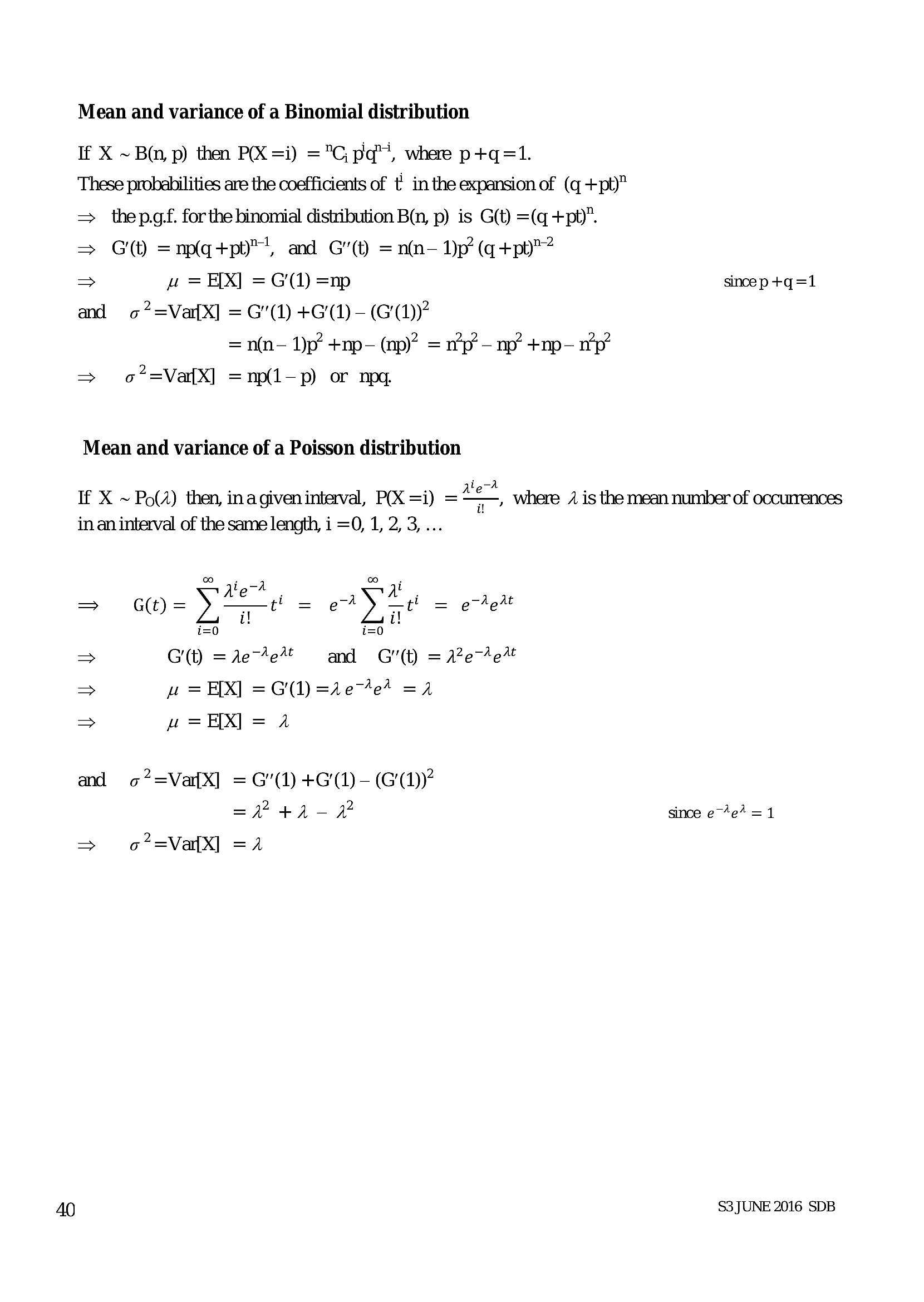
Mean and variance of a Binomial distribution If X ~B@, p) then P(X =i) ="C,pq"’, where pt+q=1. These probabilities are the coefficients of t in the expansion of (q +pt)” = thepgf. forthe binomial distribution B(n, p) is G(t) =(q +pt)”. = CW =npq+py", and G') =nlfn- Dp (q+pb"? > # = EX] =G(1) =np sincep +q=1 and o*=Vai{X] = G"(1) +G(1)- (G')” = n(n— 1)p’ +np- (np)* = n’p’— np? +np- np” o*=Va{X] =np(l-p) or nog.

Mean and variance of a Poisson distribution

ip-A
a < , Where / is the mean number of occurrences

If X ~ Po(/) then, inagiven interval, P(X =i) =
in an interval of the same length, i =0, 1, 2, 3, ...

ina

Aiea Sai
G(t) = » ~~ = ay {f= eredt
i! i!

i=0 i=0
> G(t) =Aee**# and G'(t) =12e%e%
> w= EX] =G(1) =re7e4 =2
> uw =X] = a

and o?=VarX] = G"(1) +G(1) - (GM)?
=? 41-77 since e~te? =1

o*=Vaf{X] =24

S3 JUNE 2016 SDB

---

Page 43

Extracted Text

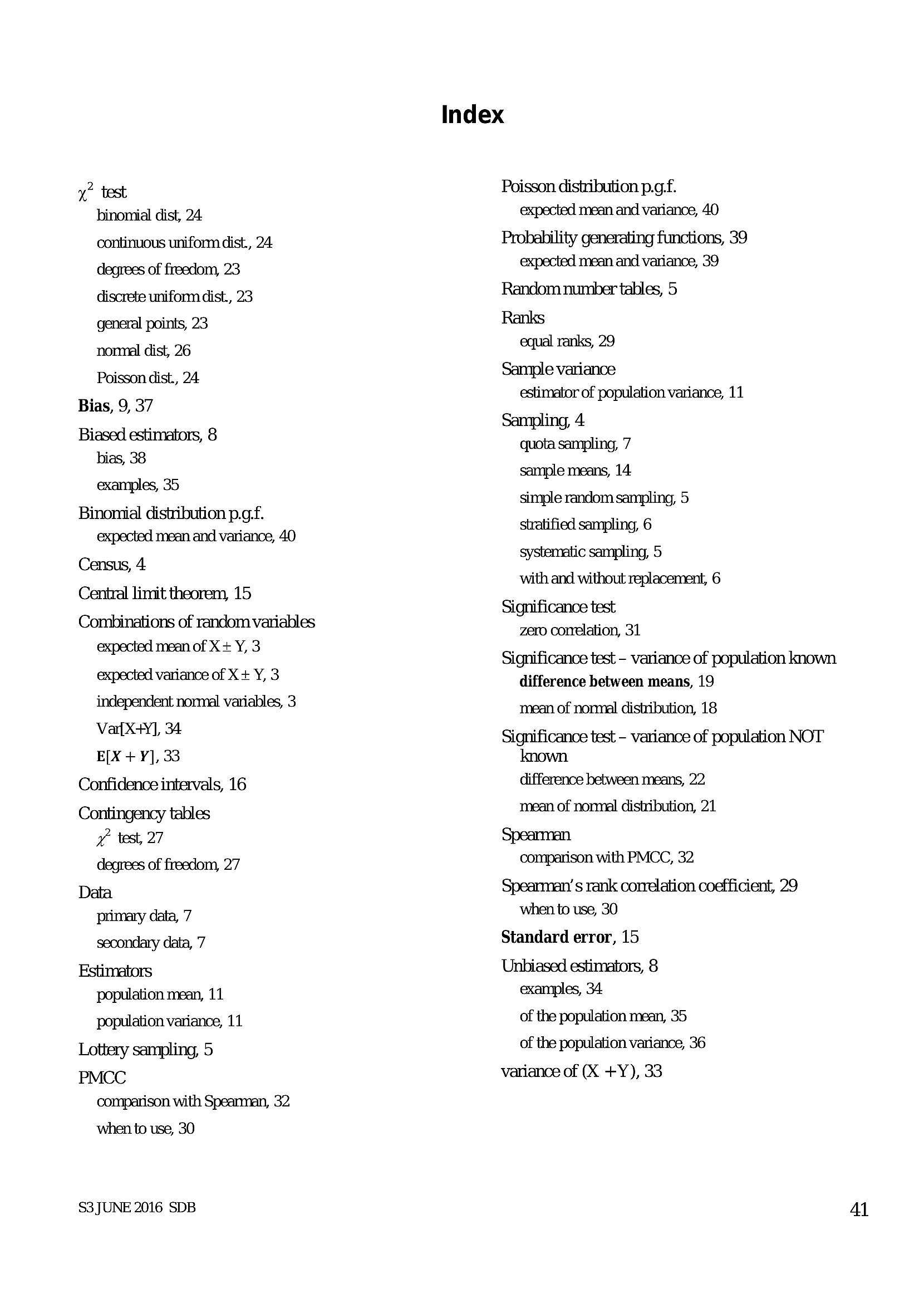
x test binomial dist, 24 continuous uniform dist., 24. degrees of freedom, 23 discrete unifonn dist., 23 general points, 23 nonmal dist, 26 Poisson dist., 24 Bias, 9, 37 Biased estimators, 8 bias, 38 examples, 35 Binomial distribution p.g.f. expected mean and variance, 40 Census, 4 Central limit theorem, 15 Combinations of random variables expected mean of X + Y, 3 expected variance of X + Y, 3 independent normal variables, 3 VarX-+Y], 34 E[X + Y], 33 Confidence intervals, 16 Contingency tables

test, 27

degrees of freedom, 27 Data primary data, 7 secondary data, 7 Estimators population mean, 11 population variance, 11 Lottery sampling, 5 PMCC comparison with Spearman, 32 when to use, 30

S3 JUNE 2016 SDB

Index

Poisson distribution p.g.f.
expected mean and variance, 40
Probability generating functions, 39
expected mean and variance, 39
Random number tables, 5
Ranks
equal ranks, 29
Sample variance
estimator of population variance, 11
Sampling, 4
quota sampling, 7
sample means, 14:
simple random sampling, 5
stratified sampling, 6
systematic sampling, 5
with and without replacement, 6
zero conelation, 31
Significance test - variance of population known
difference between means, 19
mean of normal distribution, 18
Significance test - variance of population NOT
known
difference between means, 22
mean of normal distribution, 21
Spearman
comparison with PMCC, 32
Spearman's rank correlation coefficient, 29
when to use, 30
Standard error, 15
Unbiased estimators, 8
examples, 34
of the population mean, 35
of the population variance, 36
variance of (X +Y), 33

4l

---